Cloud-Based Remote Sensing with Google Earth Engine

Fundamentals and Applications

Part F3: Advanced Image Processing

Once you understand the basics of processing images in Earth Engine, this Part will present some of the more advanced processing tools available for treating individual images. These include creating regressions among image bands, transforming images with pixel-based and neighborhood-based techniques, and grouping individual pixels into objects that can then be classified.

Chapter F3.1: Advanced Pixel-Based Image Transformation

Authors

Karen Dyson, Andréa Puzzi Nicolau, Nicholas Clinton, and David Saah

Overview

Using bands and indices is often not sufficient for obtaining high-quality image classifications. This chapter introduces the idea of more complex pixel-based band manipulations that can extract more information for analysis, building on what was presented in Part F1 and Part F2. We will first learn how to manipulate images with expressions and then move on to more complex linear transformations that leverage matrix algebra.

Learning Outcomes

• Understanding what linear transformations are and why pixel-based image transformations are useful.
• Learning how to use expressions for band manipulation.
• Being introduced to some of the most common types of linear transformations.
• Using arrays and functions in Earth Engine to apply linear transformations to images.

Assumes you know how to:

• Import images and image collections, filter, and visualize (Part F1).
• Perform basic image analysis: select bands, compute indices, create masks (Part F2).
• Use drawing tools to create points, lines, and polygons (Chap. F2.1)
• Understand basic operations of matrices

Github Code link for all tutorials

This code base is collection of codes that are freely available from different authors for google earth engine.

Github Source

Introduction to Theory

Image transformations are essentially complex calculations among image bands that can leverage matrix algebra and more advanced mathematics. In return for their greater complexity, they can provide larger amounts of information in a few variables, allowing for better classification (Chap. F2.1), time-series analysis (Chaps. F4.5 through F4.9), and change detection (Chap. F4.4) results. They are particularly useful for difficult use cases, such as classifying images with heavy shadow or high values of greenness, and distinguishing faint signals from forest degradation.

In this chapter, we explore linear transformations, which are linear combinations of input pixel values. This approach is pixel-based—that is, each pixel in the remote sensing image is treated separately.

We introduce here some of the best-established linear transformations used in remote sensing (e.g., tasseled cap transformations) along with some of the newest (e.g., spectral unmixing). Researchers are continuing to develop new applications of these methods. For example, when used together, spectral unmixing and time-series analysis (Chaps. F4.5 through F4.9) are effective at detecting and monitoring tropical forest degradation (Bullock et al. 2020). As forest degradation is notoriously hard to monitor and also responsible for significant carbon emissions, this represents an important step forward. Similarly, using tasseled cap transformations alongside classification approaches allowed researchers to accurately map cropping patterns with high spatial and thematic resolution (Rufin et al. 2019). 

Practicum

In this practicum, we will first learn how to manipulate images with expressions and then move on to more complex linear transformations that leverage matrix algebra. In Earth Engine, these types of linear transformations are applied by treating pixels as arrays of band values. An array in Earth Engine is a list of lists, and by using arrays you can define matrices (i.e., two-dimensional arrays), which are the basis of linear transformations. Earth Engine uses the word “axis” to refer to what are commonly called the rows (axis 0) and columns (axis 1) of a matrix.

Section 1. Manipulating Images with Expressions

If you have not already done so, be sure to add the book’s code repository to the Code Editor by entering https://code.earthengine.google.com/?accept_repo=projects/gee-edu/book into your browser. The book’s scripts will then be available in the script manager panel. If you have trouble finding the repo, you can visit this link for help.

Arithmetic calculation of EVI

The Enhanced Vegetation Index (EVI) is designed to minimize saturation and other issues with NDVI, an index discussed in detail in Chap. F2.0 (Huete et al. 2002). In areas of high chlorophyll (e.g., rainforests), EVI does not saturate (i.e., reach maximum value) the same way that NDVI does, making it easier to examine variation in the vegetation in these regions. The generalized equation for calculating EVI is:

         (F3.1.1)

where G, C1, C2, and L are constants. You do not need to memorize these values, as they have been determined by other researchers and are available online for you to look up. For Sentinel 2, the equation is:

         (F3.1.2)

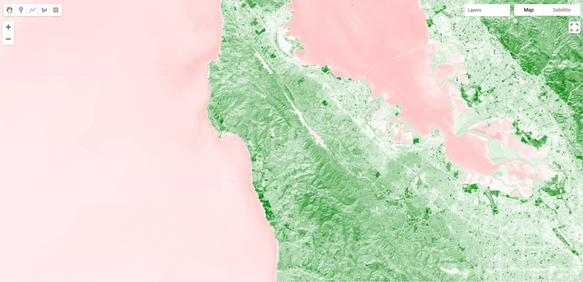
Using the basic arithmetic we learned previously in F2.0, let’s calculate and then display the EVI for the Sentinel-2 image. We will need to extract the bands and then divide by 10000 to account for the scaling in the dataset. You can find out more by navigating to the dataset information.

Using an Expression to Calculate EVI

The EVI code works (Fig. F3.1.1), but creating a large number of variables and explicitly calling addition, subtraction, multiplication, and division can be confusing and introduces the chance for errors. In these circumstances, you can create a function to make the steps more robust and easily repeatable. In another simple strategy outlined below, Earth Engine has a way to define an expression to achieve the same result.

The expression is defined first as a string using human readable names. We then define these names by selecting the proper bands.

Code Checkpoint F31a. The book’s repository contains a script that shows what your code should look like at this point.

Using an Expression to Calculate BAI

Now that we’ve seen how expressions work, let’s use an expression to calculate another index. Martin (1998) developed the Burned Area Index (BAI) to assist in the delineation of burn scars and assessment of burn severity. It relies on fires leaving ash and charcoal; fires that do not create ash or charcoal and old fires where the ash and charcoal has been washed away or covered will not be detected well. BAI computes the spectral distance of each pixel to a spectral reference point that burned areas tend to be similar to. Pixels that are far away from this reference (e.g., healthy vegetation) will have a very small value while pixels that are close to this reference (e.g., charcoal from fire) will have very large values.

        (F3.1.3)

There are two constants in this equation: ρcr  is a constant for the red band, equal to 0.1; and ρcnir is for the NIR band, equal to 0.06.

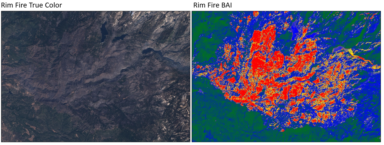
To examine burn indices, load an image from 2013 showing the Rim Fire in the Sierra Nevada, California mountains. We’ll use Landsat 8 to explore this fire. Enter the code below in a new script.

Examine the true-color display of this image. Can you spot the fire? If not, the BAI may help. As with EVI, use an expression to compute BAI in Earth Engine, using the equation above and what you know about Landsat 8 bands:

Display the result.

The burn area should be more obvious in the BAI visualization (Fig. F3.1.2, right panel). Note that the minimum and maximum values here are larger than what we have used for Landsat. At any point you can inspect a layer's bands using what you have already learned to see the minimum and maximum values, which will give you an idea of what to use here.

Code Checkpoint F31b. The book’s repository contains a script that shows what your code should look like at this point.

Section 2. Manipulating Images with Matrix Algebra

Now that we’ve covered expressions, let’s turn our attention to linear transformations that leverage matrix algebra.

Tasseled Cap Transformation

The first of these is the tasseled cap (TC) transformation. TC transformations are a class of transformations which, when graphed, look like a wooly hat with a tassel. The most common implementation is used to maximize the separation between different growth stages of wheat, an economically important crop. As wheat grows, the field progresses from bare soil, to green plant development, to yellow plant ripening, to field harvest. Separating these stages for many fields over a large area was the original purpose of the tasseled cap transformation.

Based on observations of agricultural land covers in the combined near-infrared and red spectral space, Kauth and Thomas (1976) devised a rotational transform of the form:

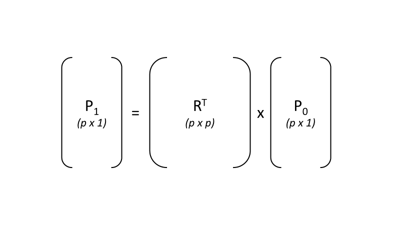
p1 =RTp0        (F3.1.4)

where p0 is the original p x 1 pixel vector (a stack of the p band values for that specific pixel as an array), and the matrix R is an orthonormal basis of the new space in which each column is orthogonal to one another (therefore RT is its transpose), and the output p1 is the rotated stack of values for that pixel (Fig. F3.1.3).

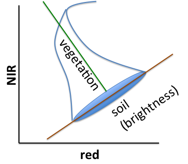
Kauth and Thomas found R by defining the first axis of their transformed space to be parallel to the soil line in Fig. F3.1.4. The first column was chosen to point along the major axis of soils and the values derived from Landsat imagery at a given point in Illinois, USA. The second column was chosen to be orthogonal to the first column and point towards what they termed “green stuff,” i.e., green vegetation. The third column is orthogonal to the first two and points towards the “yellow stuff,” e.g., ripening wheat and other grass crops. The final column is orthogonal to the first three and is called “nonesuch” in the original derivation—that is, akin to noise.

The R matrix has been derived for each of the Landsat satellites, including Landsat 5 (Crist 1985), Landsat 7, and Landsat 8, and others. We can implement this transform in Earth Engine with arrays. Specifically, let’s create a new script and make an array of TC coefficients for Landsat 5’s Thematic Mapper (TM) instrument:

Note that the structure we just made is a list of six lists, which is then converted to an Earth Engine ee.Array object. The six-by-six array of values corresponds to the linear combinations of the values of the six non-thermal bands of the TM instrument: bands 1-5 and 7. To examine how Earth Engine ingests the array, view the output of the print function to display the array in the Console. You can explore how the different elements of the array match with how the array was defined using ee.Array.

The next steps of this lab center on the small town of Odessa in eastern Washington, USA. You can search for “Odessa, WA, USA” in the search bar. We use the state abbreviation here because this is how Earth Engine displays it. The search will take you to the town and its surroundings, which you can explore with the Map or Satellite options in the upper right part of the display. In the code below, we will define a point in Odessa and center the display on it to view the results at a good zoom level.

Since these coefficients are for the TM sensor at satellite reflectance (top of atmosphere), we will access a less-cloudy Landsat 5 scene. We will access the collection of Landsat 5 images, filter them, then sort by increasing cloud cover and take the first one.

To do the matrix multiplication, first convert the input image from a multi-band image (where for each band, each pixel stores a single value) to an array image. An array image is a higher-dimension image in which each pixel stores an array of values for a band. (Array images are encountered and discussed in more detail in part F4.) You will use bands 1–5 and 7 and the toArray function:

The 1 refers to the columns (the “first” axis in Earth Engine) to create a 6 row by 1 column array for p0 (Fig. F3.1.3).

Next, we complete the matrix multiplication of the tasseled cap linear transformation using the matrixMultiply function, then convert the result back to a multi-band image using the arrayProject and arrayFlatten functions:

Finally, display the result:

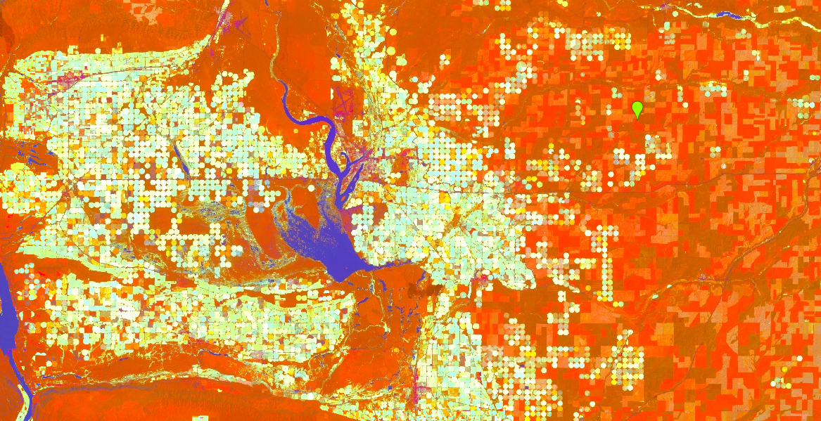
This maps brightness to red, greenness to green, and wetness to blue. Your resulting layer will contain a high amount of contrast (Fig. F3.1.5). Water appears blue, healthy irrigated crops are the bright circles, and drier crops are red. We have chosen this area near Odessa because it is naturally dry, and the irrigated crops make the patterns identified by the tasseled cap transformation particularly striking.

If you would like to see how the array image operations work, you can consider building tasselCapImage, one step at a time. You can assign the result of matrixMultiply operation to its own variable, then map the result. Then, do the arrayProject command on that new variable into a second new image, and map that result. Then, do the arrayFlatten call on that result to produce tasselCapImage as before. You can then use the Inspector tool to view these details of how the data is processed as tasselCapImage is built.

Principal Component Analysis

Like the TC transform, the principal component analysis (PCA) transform is a rotational transform. PCA is an orthogonal linear transformation—essentially, it mathematically transforms the data into a new coordinate system where all axes are orthogonal. The first axis, also called a coordinate, is calculated to capture the largest amount of variance of the dataset, the second captures the second-greatest variance, and so on.

Because these are calculated to be orthogonal, the principal components are uncorrelated. PCA can be used as a dimension reduction tool, as most of the variation in a dataset with n axes can be captured in n − x axes. This is a very brief explanation; if you want to learn more about PCA and how it works, there are many excellent statistical texts and online resources on the subject.

To demonstrate the practical application of PCA applied to an image, import the Landsat 8 TOA image, and name it imageL8. First, we will convert it to an array image:

In the next step, use the reduceRegion method and the ee.Reducer.covariance function to compute statistics (in this case the covariance of bands) for the image.

Note that the result of the reduction is an object with one property, array, that stores the covariance matrix. We use the ee.Array.get function to extract the covariance matrix and store it as an array.

Now that we have a covariance matrix based on the image, we can perform an eigen analysis to compute the eigenvectors that we will need to perform the PCA. To do this, we will use the eigen function. Again, if these terms are unfamiliar to you, we suggest one of the many excellent statistics textbooks or online resources. Compute the eigenvectors and eigenvalues of the covariance matrix:

The eigen function outputs both eigenvectors and the eigenvalues. Since we need the eigenvectors for the PCA, we can use the slice function for arrays to extract them. The eigenvectors are stored in the 0th position of the 1 axis.

Now we perform matrix multiplication using these eigenVectors and the arrayImage we created earlier. This is the same process that we used with the tasseled cap components. Each multiplication results in a principal component.

Finally, convert back to a multi-band image and display the first principal component (pc1):

When first displayed, the PC layer will be all black. Use the layer manager to stretch the result in greyscale by hovering over Layers, then PC, and then clicking the gear icon next to PC. Note how the range (minimum and maximum values) changes based on the stretch you choose.

What do you observe? Try displaying some of the other principal components. How do they differ from each other? What do you think each band is capturing? Hint: You will need to recreate the stretch for each principal component you try to map.

Look at what happens when you try to display 'pc1', 'pc3', and 'pc4', for example, in a three-band display. Because the values of each principal component band differ substantially, you might see a gradation of only one color in your output. To control the display of multiple principal component bands together, you will need to use lists in order to specify the min and max values individually for each principal component band.

Once you have determined which bands you would like to plot, input the min and max values for each band, making sure they are in the correct order.

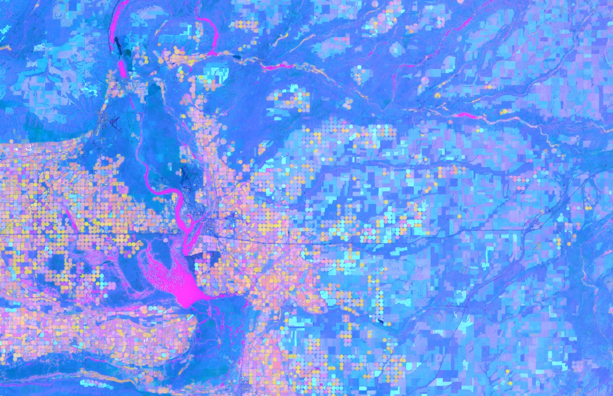
Examine the PCA map (Fig. F3.1.6). Unlike with the tasseled cap transformation, PCA does not have defined output axes. Instead, each axis dynamically captures some aspect of the variation within the dataset (if this does not make sense to you, please review an online resource on the statistical theory behind PCA). Thus, the mapped PCA may differ substantially based on where you have performed the PCA and which bands you are mapping.

Code Checkpoint F31c. The book’s repository contains a script that shows what your code should look like at this point.

Section 3. Spectral Unmixing 

If we think about a single pixel in our dataset—a 30 m x 30 m space corresponding to a Landsat pixel, for instance—it is likely to represent multiple physical objects on the ground. As a result, the spectral signature for the pixel is a mixture of the “pure” spectra of each object existing in that space. For example, consider a Landsat pixel of forest. The spectral signature of the pixel is a mixture of trees, understory, shadows cast by the trees, and patches of soil visible through the canopy.

The linear spectral unmixing model is based on this assumption. The pure spectra, called endmembers, are from land cover classes such as water, bare land, and vegetation. These endmembers represent the spectral signature of pure spectra from ground features, such as only bare ground. The goal is to solve the following equation for ƒ, the P x 1 vector of endmember fractions in the pixel:

        (F3.1.5)

S is a B x P matrix in which B is the number of bands and the columns are P pure endmember spectra and p is the B x 1 pixel vector when there are B bands (Fig. F3.1.7). We know p and we can define the endmember spectra to get S such that we can solve for ƒ.

We’ll use the Landsat 8 image for this exercise. In this example, the number of bands (B) is six.

The first step is to define the endmembers such that we can define S. We will do this by computing the mean spectra in polygons delineated around regions of pure land cover.

Zoom the map to a location with homogeneous areas of bare land, vegetation, and water (an airport can be used as a suitable location). Visualize the Landsat 8 image as a false color composite:

For faster rendering, you may want to comment out previous layers you added to the map.

In general, the way to do this is to draw polygons around areas of pure land cover in order to define the spectral signature of these land covers. If you’d like to do this on your own, here’s how. Using the geometry drawing tools, make three new layers (thus, P =3) by selecting the polygon tool and then clicking + new layer. In the first layer, digitize a polygon around pure bare land; in the second layer, make a polygon of pure vegetation; in the third layer, make a water polygon. Name the imports bare, water, and veg, respectively. You will need to use the settings (gear icon) to rename the geometries.

You can also use this code to specify predefined areas of bare, water, and vegetation. This will only work for this example.

Check the polygons you made or imported by charting mean spectra in them using ui.Chart.image.regions.

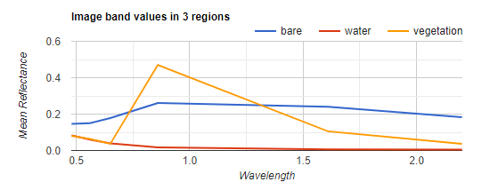
The xLabels line of code takes the mean of each polygon (feature) at the spectral midpoint of each of the six bands. The numbers ([0.48, 0.56, 0.65, 0.86, 1.61, 2.2]) represent these spectral midpoints. Your chart should look something like Fig. F3.1.8.

Use the reduceRegion method to compute the mean values within the polygons you made, for each of the bands. Note that the return value of reduceRegion is a Dictionary of numbers summarizing values within the polygons, with the output indexed by band name.

Get the means as a List by calling the values function after computing the mean. Note that values returns the results in alphanumeric order sorted by the keys. This works because B2–B7 are already alphanumerically sorted, but it will not work in cases when they are not already sorted. In those cases, please specify the list of band names so that you get them in a known order first.

Each of these three lists represents a mean spectrum vector, which is one of the columns for our S matrix defined above. Stack the vectors into a 6 x 3 Array of endmembers by concatenating them along the 1-axis (columns):

Use print if you would like to view your new matrix.

As we have done in previous sections, we will now convert the 6-band input image into an image in which each pixel is a 1D vector (toArray), then into an image in which each pixel is a 6 x 1 matrix (toArray(1)). This creates p so that we can solve the equation above for each pixel.

Now that we have everything in place, for each pixel we solve the equation for ƒ:

For this task, we use the matrixSolve function. This function solves for x in the equation . Here, A is our matrix S and B is the matrix p.

Finally, convert the result from a two-dimensional array image into a one-dimensional array image (arrayProject), and then into a zero-dimensional, more familiar multi-band image (arrayFlatten). This is the same approach we used in previous sections. The three bands correspond to the estimates of bare, vegetation, and water fractions in ƒ:

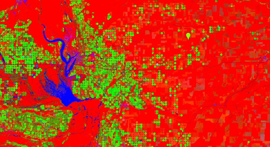
Display the result where bare is red, vegetation is green, and water is blue (the addLayer call expects bands in order, RGB). Use either code or the layer visualization parameter tool to achieve this. Your resulting image should look like Fig. F3.1.9.

Section 4. The Hue, Saturation, Value Transform

Whereas the other three transforms we have discussed will transform the image based on spectral signatures from the original image, the hue, saturation, value (HSV) transform is a color transform of the RGB color space.

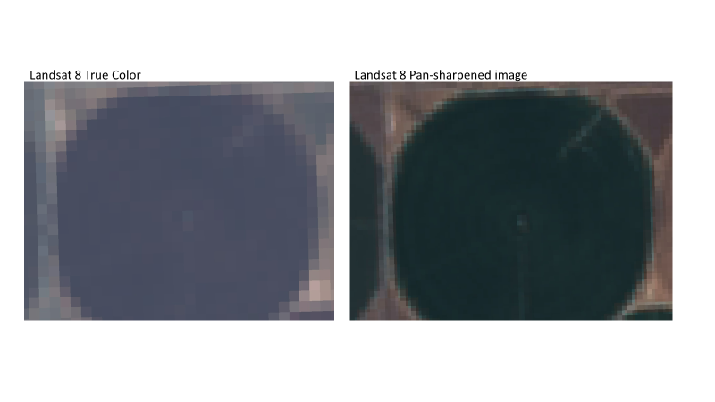
Among many other things, it is useful for pan-sharpening, a process by which a higher-resolution panchromatic image is combined with a lower-resolution multiband raster. This involves converting the multiband raster RGB to HSV color space, swapping the panchromatic band for the value band, then converting back to RGB. Because the value band describes the brightness of colors in the original image, this approach leverages the higher resolution of the panchromatic image.

For example, let’s pansharpen the Landsat 8 scene we have been working with in this chapter. In Landsat 8, the panchromatic band is 15 m resolution while the RGB bands are 30 m resolution. We use the rgbToHsv function here—it is such a common transform that there is a built-in function for it.

Next we convert the image back to RGB space after substituting the panchromatic band for the Value band, which appears third in the HSV image. We do this by first concatenating the different image bands using the ee.Image.cat function, and then by converting to RGB.

In Fig. F3.1.10, compare the pan-sharpened image to the original true-color image. What do you notice? Is it easier to interpret the image following pan-sharpening?

Code Checkpoint F31d. The book’s repository contains a script that shows what your code should look like at this point.

Synthesis

Assignment 1. Write an expression to calculate the Normalized Burn Ratio Thermal (NBRT) index for the Rim Fire Landsat 8 image (burnImage).

NBRT was developed based on the idea that burned land has low NIR reflectance (less vegetation), high SWIR reflectance (from ash, etc.), and high brightness temperature (Holden et al. 2005).

The formula is:

        (F3.1.6)

Where NIR should be between 0.76 to 0.9 µm, SWIR 2.08 to 2.35 µm, and Thermal 10.4 to 12.5 µm.

To display this result, remember that a lower NBRT is the result of more burning.

Bonus: Here’s another way to reverse a color palette (note the min and max values):

The difference in this index, before compared with after the fire, can be used as a diagnostic of burn severity (see van Wagtendonk et al. 2004).

Conclusion

Linear image transformations are a powerful tool in remote sensing analysis. By choosing your linear transformation carefully, you can highlight specific aspects of your data that make image classification easier and more accurate. For example, spectral unmixing is frequently used in change detection applications like detecting forest degradation. By using the endmembers (pure spectra) as inputs to the change detection algorithms, the model is better able to detect subtle changes due to the removal of some but not all the trees in the pixel.

Feedback

To review this chapter and make suggestions or note any problems, please go now to bit.ly/EEFA-review. You can find summary statistics from past reviews at bit.ly/EEFA-reviews-stats.

References

Cloud-Based Remote Sensing with Google Earth Engine. (n.d.). CLOUD-BASED REMOTE SENSING WITH GOOGLE EARTH ENGINE. https://www.eefabook.org/

Cloud-Based Remote Sensing with Google Earth Engine. (2024). In Springer eBooks. https://doi.org/10.1007/978-3-031-26588-4

Baig MHA, Zhang L, Shuai T, Tong Q (2014) Derivation of a tasselled cap transformation based on Landsat 8 at-satellite reflectance. Remote Sens Lett 5:423–431. https://doi.org/10.1080/2150704X.2014.915434

Bullock EL, Woodcock CE, Olofsson P (2020) Monitoring tropical forest degradation using spectral unmixing and Landsat time series analysis. Remote Sens Environ 238:110968. https://doi.org/10.1016/j.rse.2018.11.011

Crist EP (1985) A TM tasseled cap equivalent transformation for reflectance factor data. Remote Sens Environ 17:301–306. https://doi.org/10.1016/0034-4257(85)90102-6

Drury SA (1987) Image interpretation in geology. Geocarto Int 2:48. https://doi.org/10.1080/10106048709354098

Gao BC (1996) NDWI - A normalized difference water index for remote sensing of vegetation liquid water from space. Remote Sens Environ 58:257–266. https://doi.org/10.1016/S0034-4257(96)00067-3

Holden ZA, Smith AMS, Morgan P, et al (2005) Evaluation of novel thermally enhanced spectral indices for mapping fire perimeters and comparisons with fire atlas data. Int J Remote Sens 26:4801–4808. https://doi.org/10.1080/01431160500239008

Huang C, Wylie B, Yang L, et al (2002) Derivation of a tasselled cap transformation based on Landsat 7 at-satellite reflectance. Int J Remote Sens 23:1741–1748. https://doi.org/10.1080/01431160110106113

Huete A, Didan K, Miura T, et al (2002) Overview of the radiometric and biophysical performance of the MODIS vegetation indices. Remote Sens Environ 83:195–213. https://doi.org/10.1016/S0034-4257(02)00096-2

Jackson RD, Huete AR (1991) Interpreting vegetation indices. Prev Vet Med 11:185–200. https://doi.org/10.1016/S0167-5877(05)80004-2

Martín MP (1998) Cartografía e inventario de incendios forestales en la Península Ibérica a partir de imágenes NOAA-AVHRR. Universidad de Alcalá

McFeeters SK (1996) The use of the Normalized Difference Water Index (NDWI) in the delineation of open water features. Int J Remote Sens 17:1425–1432. https://doi.org/10.1080/01431169608948714

Nath B, Niu Z, Mitra AK (2019) Observation of short-term variations in the clay minerals ratio after the 2015 Chile great earthquake (8.3 Mw) using Landsat 8 OLI data. J Earth Syst Sci 128:1–21. https://doi.org/10.1007/s12040-019-1129-2

Rufin P, Frantz D, Ernst S, et al (2019) Mapping cropping practices on a national scale using intra-annual Landsat time series binning. Remote Sens 11:232. https://doi.org/10.3390/rs11030232

Schultz M, Clevers JGPW, Carter S, et al (2016) Performance of vegetation indices from Landsat time series in deforestation monitoring. Int J Appl Earth Obs Geoinf 52:318–327. https://doi.org/10.1016/j.jag.2016.06.020

Segal D (1982) Theoretical basis for differentiation of ferric-iron bearing minerals, using Landsat MSS data. In: Proceedings of Symposium for Remote Sensing of Environment, 2nd Thematic Conference on Remote Sensing for Exploratory Geology, Fort Worth, TX. pp 949–951

Souza Jr CM, Roberts DA, Cochrane MA (2005) Combining spectral and spatial information to map canopy damage from selective logging and forest fires. Remote Sens Environ 98:329–343. https://doi.org/10.1016/j.rse.2005.07.013

Souza Jr CM, Siqueira JV, Sales MH, et al (2013) Ten-year landsat Classification of deforestation and forest degradation in the Brazilian Amazon. Remote Sens 5:5493–5513. https://doi.org/10.3390/rs5115493

Van Wagtendonk JW, Root RR, Key CH (2004) Comparison of AVIRIS and Landsat ETM+ detection capabilities for burn severity. Remote Sens Environ 92:397–408. https://doi.org/10.1016/j.rse.2003.12.015