Cloud-Based Remote Sensing with Google Earth Engine

Fundamentals and Applications

Part F5: Vectors and Tables

In addition to raster data processing, Earth Engine supports a rich set of vector processing tools. This Part introduces you to the vector framework in Earth Engine, shows you how to create and to import your vector data, and how to combine vector and raster data for analyses.

Chapter F5.1: Raster/Vector Conversions

Authors

Keiko Nomura, Samuel Bowers

Overview 

The purpose of this chapter is to review methods of converting between raster and vector data formats, and to understand the circumstances in which this is useful. By way of example, this chapter focuses on topographic elevation and forest cover change in Colombia, but note that these are generic methods that can be applied in a wide variety of situations.

Learning Outcomes

• Understanding raster and vector data in Earth Engine and their differing properties.
• Knowing how and why to convert from raster to vector.
• Knowing how and why to convert from vector to raster.
• Write a function and map it over a FeatureCollection.

Assumes you know how to:

• Import images and image collections, filter, and visualize (Part F1).
• Understand distinctions among Image, ImageCollection, Feature and FeatureCollection Earth Engine objects (Part F1, Part F2, Part F5).
• Perform basic image analysis: select bands, compute indices, create masks (Part F2).
• Perform image morphological operations (Chap. F3.2).
• Understand the filter, map, reduce paradigm (Chap. F4.0).
• Write a function and map it over an ImageCollection (Chap. F4.0).
• Use reduceRegions to summarize an image in irregular shapes (Chap. F5.0).

Github Code link for all tutorials

This code base is collection of codes that are freely available from different authors for google earth engine.

Github Source

Introduction to Theory

Raster data consists of regularly spaced pixels arranged into rows and columns, familiar as the format of satellite images. Vector data contains geometry features (i.e., points, lines, and polygons) describing locations and areas. Each data format has its advantages, and both will be encountered as part of GIS operations.

Raster and vector data are commonly combined (e.g., extracting image information for a given location or clipping an image to an area of interest); however, there are also situations in which conversion between the two formats is useful. In making such conversions, it is important to consider the key advantages of each format. Rasters can store data efficiently where each pixel has a numerical value, while vector data can more effectively represent geometric features where homogenous areas have shared properties. Each format lends itself to distinctive analytical operations, and combining them can be powerful.

In this exercise, we’ll use topographic elevation and forest change images in Colombia as well as a protected area feature collection to practice the conversion between raster and vector formats, and to identify situations in which this is worthwhile.

Practicum

Section 1. Raster to Vector Conversion 

Section 1.1. Raster to Polygons

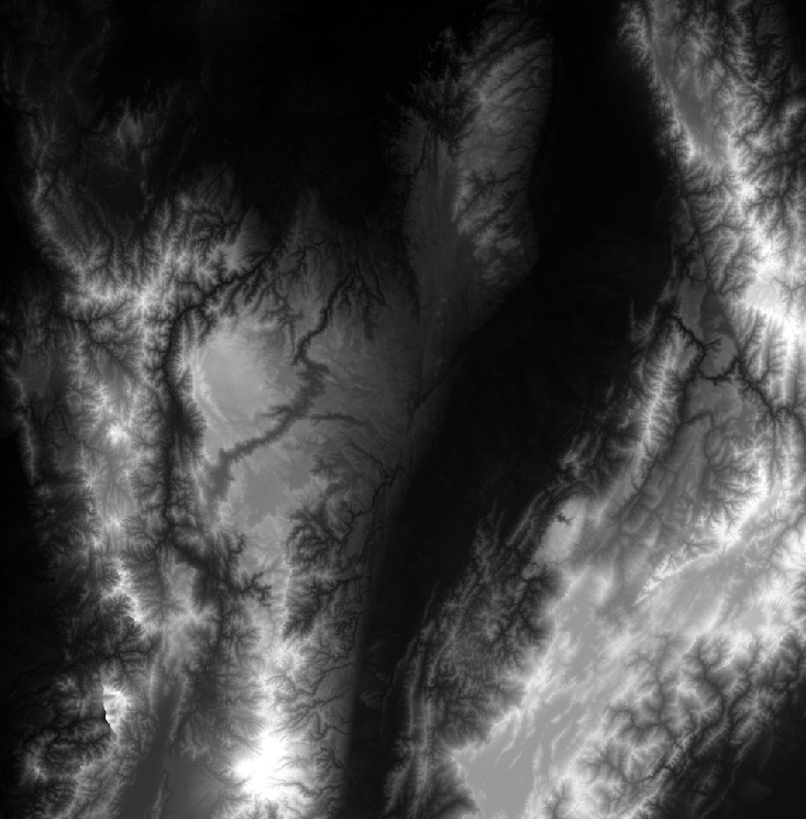
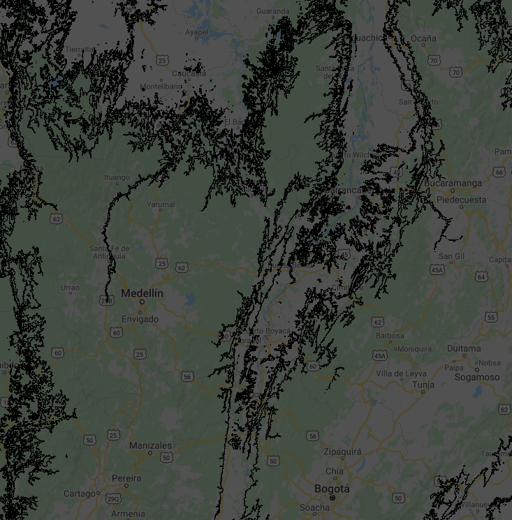
In this section we will convert an elevation image (raster) to a feature collection (vector). We will start by loading the Global Multi-Resolution Terrain Elevation Data 2010 and the Global Administrative Unit Layers 2015 dataset to focus on Colombia. The elevation image is a raster at 7.5 arc-second spatial resolution containing a continuous measure of elevation in meters in each pixel.

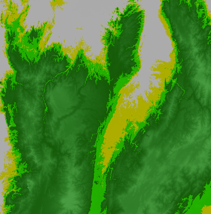
When converting an image to a feature collection, we will aggregate the categorical elevation values into a set of categories to create polygon shapes of connected pixels with similar elevations. For this exercise, we will create four zones of elevation by grouping the altitudes to 0-100 m=0, 100–200 m=1, 200–500 m=2, and >500 m=3.

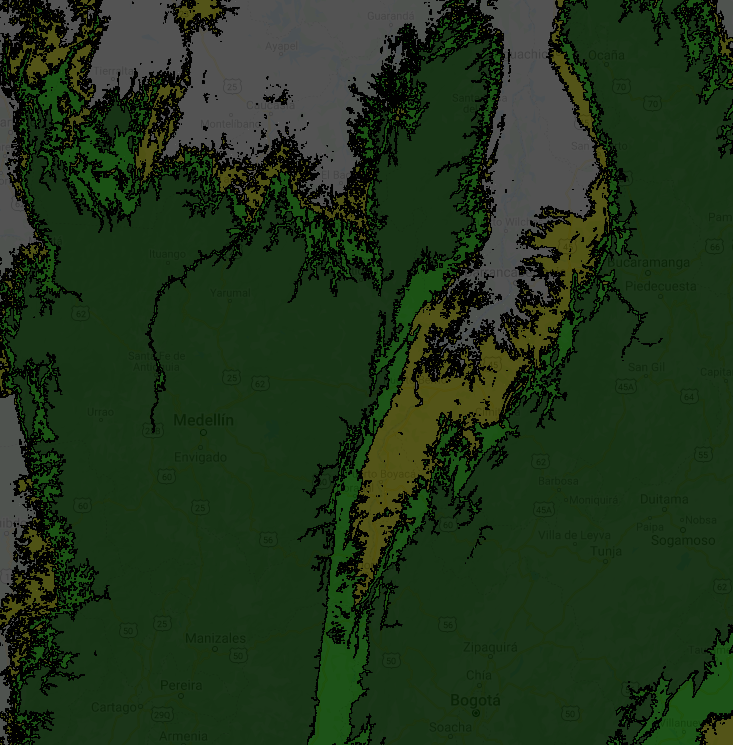
We will convert this zonal elevation image in Colombia to polygon shapes, which is a vector format (termed a FeatureCollection in Earth Engine), using the ee.Image.reduceToVectors method. This will create polygons delineating connected pixels with the same value. In doing so, we will use the same projection and spatial resolution as the image. Please note that loading the vectorized image in the native resolution (231.92 m) takes time to execute. For faster visualization, we set a coarse scale of 1,000 m.

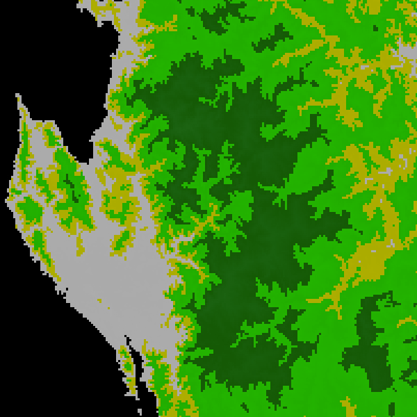
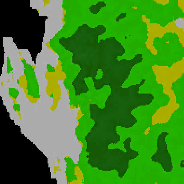
You may have realized that polygons consist of complex lines, including some small polygons with just one pixel. That happens when there are no surrounding pixels of the same elevation zone. You may not need a vector map with such details—if, for instance, you want to produce a regional or global map. We can use a morphological reducer focalMode to simplify the shape by defining a neighborhood size around a pixel. In this example, we will set the kernel radius as four pixels. This operation makes the resulting polygons look much smoother, but less precise (Fig. F5.1.2).

We can see now that the polygons have more distinct shapes with many fewer small polygons in the new map (Fig. F5.1.2). It is important to note that when you use methods like focalMode (or other, similar methods such as connectedComponents and connectedPixelCount), you need to reproject according to the original image in order to display properly with zoom using the interactive Code Editor.

Section 1.2. Raster to Points

Lastly, we will convert a small part of this elevation image into a point vector dataset. For this exercise, we will use the same example and build on the code from the previous subsection. This might be useful when you want to use geospatial data in a tabular format in combination with other conventional datasets such as economic indicators (Fig. F5.1.3).

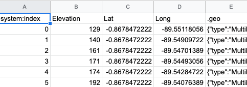
The easiest way to do this is to use sample while activating the geometries parameter. This will extract the points at the centroid of the elevation pixel.

We can also extract sample points per elevation zone. Below is an example of extracting 10 randomly selected points per elevation zone (Fig. F5.1.4). You can also set different values for each zone using classValues and classPoints parameters to modify the sampling intensity in each class. This may be useful, for instance, to generate point samples for a validation effort.

Code Checkpoint F51a. The book’s repository contains a script that shows what your code should look like at this point.

Section 1.3. A More Complex Example

In this section we’ll use two global datasets, one to represent raster formats and the other vectors:

• The Global Forest Change (GFC) dataset: a raster dataset describing global tree cover and change for 2001–present.
• The World Protected Areas Database: a vector database of global protected areas.

The objective will be to combine these two datasets to quantify rates of deforestation in protected areas in the “arc of deforestation” of the Colombian Amazon. The datasets can be loaded into Earth Engine with the following code:

The GFC dataset (first presented in detail in Chap. F1.1) is a global set of rasters that quantify tree cover and change for the period beginning in 2001. We’ll use a single image from this dataset:

• 'lossyear': a categorical raster of forest loss (1–20, corresponding to deforestation for the period 2001–2020), and 0 for no change

The World Database on Protected Areas (WDPA) is a harmonized dataset of global terrestrial and marine protected area locations, along with details on the classification and management of each. In addition to protected area outlines, we’ll use two fields from this database:

• 'NAME'’: the name of each protected area
• ‘WDPA_PID’: a unique numerical ID for each protected area

To begin with, we’ll focus on forest change dynamics in ‘La Paya’, a small protected area in the Colombian Amazon. We’ll first visualize these data using the paint command, which is discussed in more detail in Chap. F5.3:

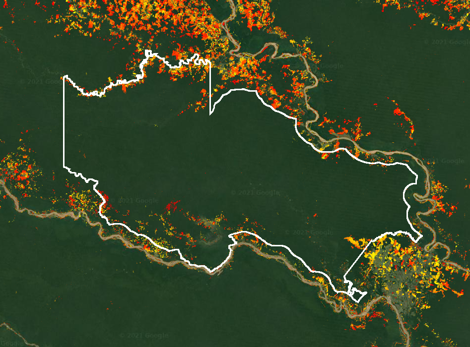
This will display the boundary of the La Paya protected area and deforestation in the region (Fig. F5.1.5).

We can use Earth Engine to convert the deforestation raster to a set of polygons. The deforestation data are appropriate for this transformation as each deforestation event is labeled categorically by year, and change events are spatially contiguous. This is performed in Earth Engine using the ee.Image.reduceToVectors method, as described earlier in this section.  

Fig. F5.1.6 shows a comparison of the raster versus vector representations of deforestation within the protected area.

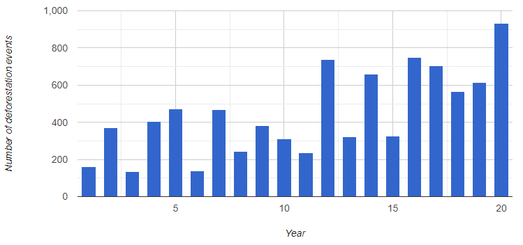
Having converted from raster to vector, a new set of operations becomes available for post-processing the deforestation data. We might, for instance, be interested in the number of individual change events each year (Fig. F5.1.7):

There might also be interest in generating point locations for individual change events (e.g., to aid a field campaign):

The vector format allows for easy filtering to only deforestation events of interest, such as only the largest deforestation events:

Code Checkpoint F51b. The book’s repository contains a script that shows what your code should look like at this point.

Section 1.4: Raster Properties to Vector Fields

Sometimes we want to extract information from a raster to be included in an existing vector dataset. An example might be estimating a deforestation rate for a set of protected areas. Rather than perform this task on a case-by-case basis, we can attach information generated from an image as a property of a feature.

The following script shows how this can be used to quantify a deforestation rate for a set of protected areas in the Colombian Amazon.

The output of this script is an estimate of deforested area in hectares for each reserve. However, as reserve sizes vary substantially by area, we can normalize by the total area of each reserve to quantify rates of change.

Code Checkpoint F51c. The book’s repository contains a script that shows what your code should look like at this point.

Section 2. Vector-to-Raster Conversion

In Sect. 1, we used the protected area feature collection as its original vector format. In this section, we will rasterize the protected area polygons to produce a mask and use this to assess rates of forest change.

Section 2.1. Polygons to a Mask

The most common operation to convert from vector to raster is the production of binary image masks, describing whether a pixel intersects a line or falls within a polygon. To convert from vector to a raster mask, we can use the ee.FeatureCollection.reduceToImage method. Let’s continue with our example of the WDPA database and Global Forest Change data from the previous section:

We can use this mask to, for example, highlight only deforestation that occurs within a protected area using logical operations:

In the above example we generated a simple binary mask, but reduceToImage can also preserve a numerical property of the input polygons. For example, we might want to be able to determine which protected area each pixel represents. In this case, we can produce an image with the unique ID of each protected area:

This output can be useful when performing large-scale raster operations, such as efficiently calculating deforestation rates for multiple protected areas.

Code Checkpoint F51d. The book’s repository contains a script that shows what your code should look like at this point.

Section 2.2. A More Complex Example

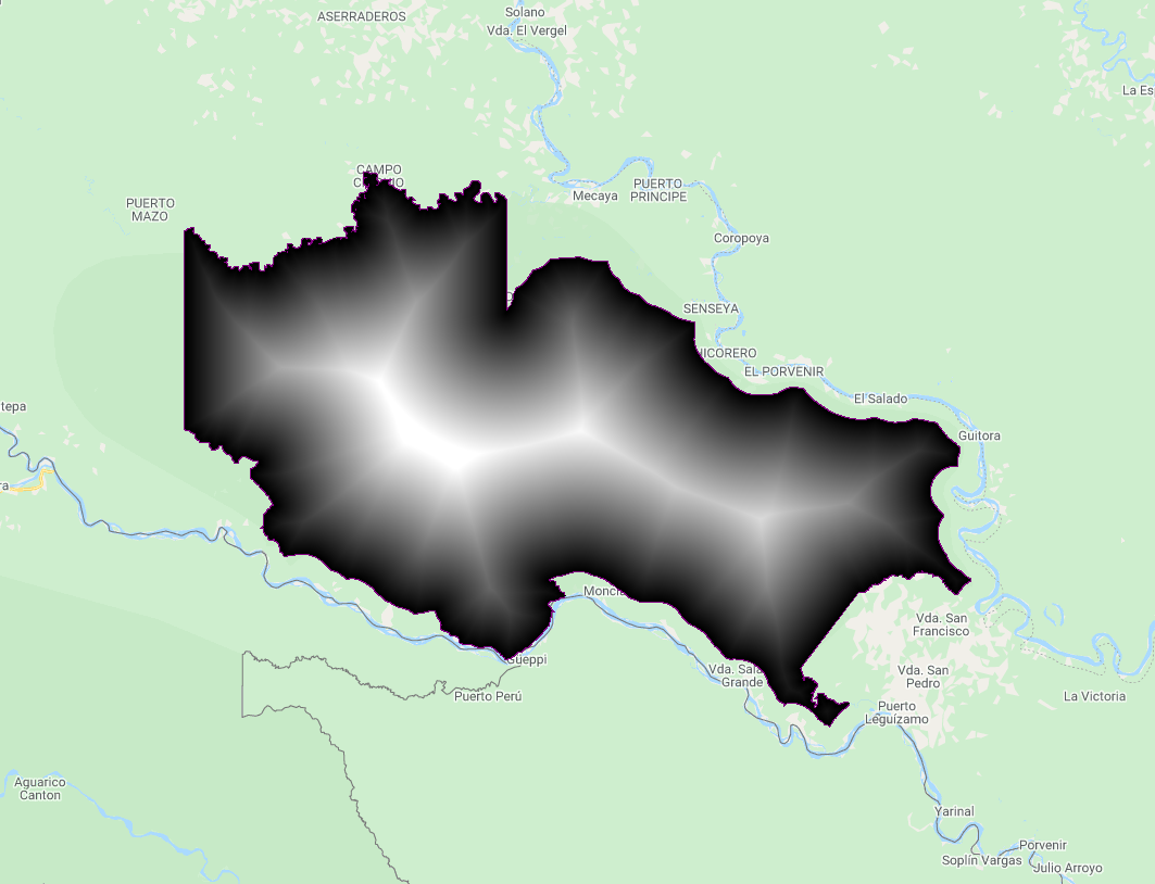
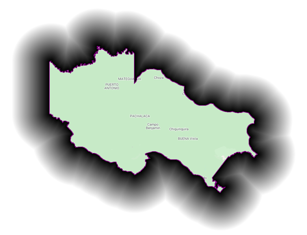
The reduceToImage method is not the only way to convert a feature collection to an image. We will create a distance image layer from the boundary of the protected area using distance. For this example, we return to the La Paya protected area explored in Sect. 1.

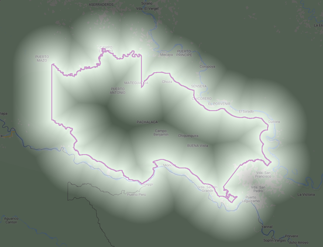
We can also show the distance inside and outside of the boundary by using the rasterized protected area (Fig. F5.1.8).

Sometimes it makes sense to work with objects in raster imagery. This is an unusual case of vector-like operations conducted with raster data. There is a good reason for this where the vector equivalent would be computationally burdensome.

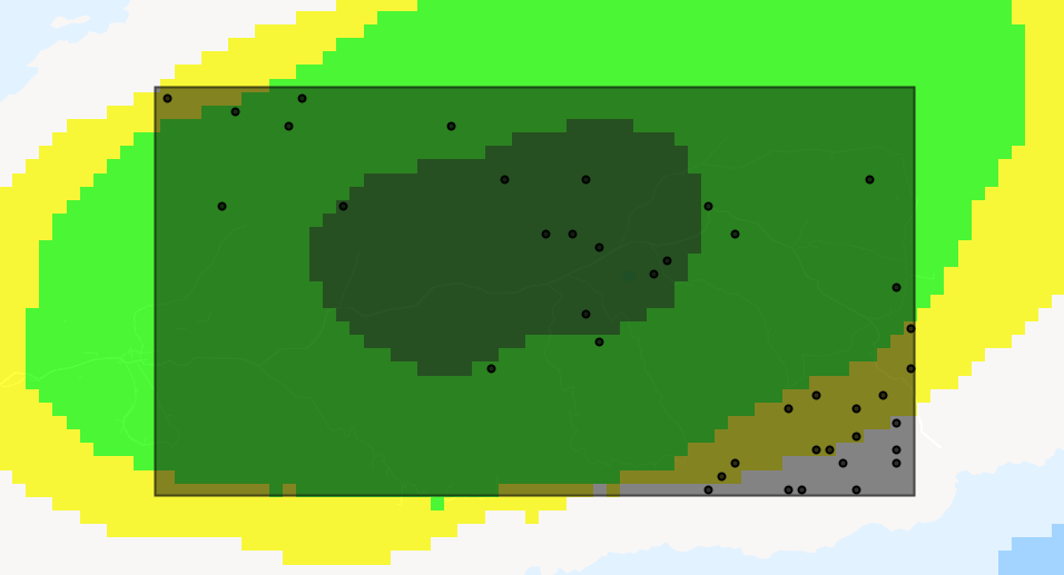
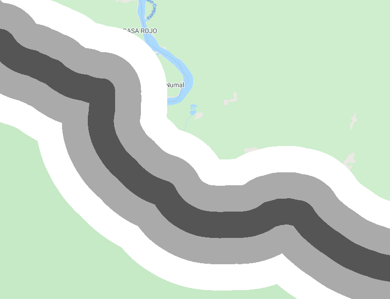
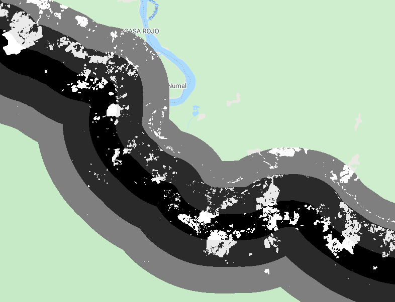
An example of this is estimating deforestation rates by distance to the edge of the protected area, as it is common that rates of change will be higher at the boundary of a protected area. We will create a distance raster with three zones from the La Paya boundary (>1 km, >2 km, >3 km, and >4 km) and to estimate the deforestation by distance from the boundary (Fig. F5.1.9).

Lastly, we can estimate the deforestation area within 1 km of the protected area but only outside of the boundary.

Code Checkpoint F51e. The book’s repository contains a script that shows what your code should look like at this point.

Synthesis

Question 1. In this lab, we quantified rates of deforestation in La Paya. There is another protected area in the Colombian Amazon named Tinigua. By modifying the existing scripts, determine how the dynamics of forest change in Tinigua compare to those in La Paya with respect to:

• the number of deforestation events
• the year with the greatest number of change events
• the mean average area of change events
• the total area of loss

Question 2. In Sect. 1.4, we only considered losses of tree cover, but many protected areas will also have increases in tree cover from regrowth (which is typical of shifting agriculture). Calculate growth in hectares using the Global Forest Change dataset’s gain layer for the six protected areas in Sect. 1.4 by extracting the raster properties and adding them to vector fields. Which has the greatest area of regrowth? Is this likely to be sufficient to balance out the rates of forest loss? Note: The gain layer shows locations where tree cover has increased for the period 2001–2012 (0=no gain, 1=tree cover increase), so for comparability use deforestation between the same time period of 2001–2012.

Question 3. In Sect. 2.2, we considered rates of deforestation in a buffer zone around La Paya. Estimate the deforestation rates inside of La Paya using buffer zones. Is forest loss more common close to the boundary of the reserve?

Question 4. Sometimes it’s advantageous to perform processing using raster operations, particularly at large scales. It is possible to perform many of the tasks in Sect. 1.3 and 1.4 by first converting the protected area vector to raster, and then using only raster operations. As an example, can you display only deforestation events >10 ha in La Paya using only raster data? (Hint: Consider using ee.Image.connectedPixelCount. You may also want to also look at Sect. 2.1).

Conclusion

In this chapter, you learned how to convert raster to vector and vice versa. More importantly, you now have a better understanding of why and when such conversions are useful. Our examples should give you practical applications and ideas for using these techniques.

Feedback

To review this chapter and make suggestions or note any problems, please go now to bit.ly/EEFA-review. You can find summary statistics from past reviews at bit.ly/EEFA-reviews-stats.

References

Cloud-Based Remote Sensing with Google Earth Engine. (n.d.). CLOUD-BASED REMOTE SENSING WITH GOOGLE EARTH ENGINE. https://www.eefabook.org/

Cloud-Based Remote Sensing with Google Earth Engine. (2024). In Springer eBooks. https://doi.org/10.1007/978-3-031-26588-4