Cloud-Based Remote Sensing with Google Earth Engine

Fundamentals and Applications

Part F2: Interpreting Images

Now that you know how images are viewed and what kinds of images exist in Earth Engine, how do we manipulate them? To gain the skills of interpreting images, you’ll work with bands, combining values to form indices and masking unwanted pixels. Then, you’ll learn some of the techniques available in Earth Engine for classifying images and interpreting the results.

Chapter F2.1: Interpreting an Image: Classification

Authors

Andréa Puzzi Nicolau, Karen Dyson, David Saah, Nicholas Clinton

Overview

Image classification is a fundamental goal of remote sensing. It takes the user from viewing an image to labeling its contents. This chapter introduces readers to the concept of classification and walks users through the many options for image classification in Earth Engine. You will explore the processes of training data collection, classifier selection, classifier training, and image classification.

Learning Outcomes

• Running a classification in Earth Engine.
• Understanding the difference between supervised and unsupervised classification.
• Learning how to use Earth Engine geometry drawing tools.
• Learning how to collect sample data in Earth Engine.
• Learning the basics of the hexadecimal numbering system.

Assumes you know how to:

• Import images and image collections, filter, and visualize (Part F1).
• Understand bands and how to select them (Chap. F1.2, Chap. F2.0).

Github Code link for all tutorials

This code base is collection of codes that are freely available from different authors for google earth engine.

Github Source

Introduction to Theory

Classification is addressed in a broad range of fields, including mathematics, statistics, data mining, machine learning, and more. For a deeper treatment of classification, interested readers may see some of the following suggestions: Witten et al. (2011), Hastie et al. (2009), Goodfellow et al. (2016), Gareth et al. (2013), Géron (2019), Müller et al. (2016), or Witten et al. (2005). Unlike regression, which predicts continuous variables, classification predicts categorical, or discrete, variables—variables with a finite number of categories (e.g., age range).

In remote sensing, image classification is an attempt to categorize all pixels in an image into a finite number of labeled land cover and/or land use classes. The resulting classified image is a simplified thematic map derived from the original image (Fig. F2.1.1). Land cover and land use information is essential for many environmental and socioeconomic applications, including natural resource management, urban planning, biodiversity conservation, agricultural monitoring, and carbon accounting.

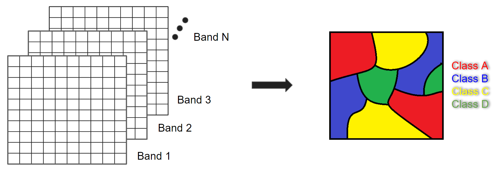
Image classification techniques for generating land cover and land use information have been in use since the 1980s (Li et al. 2014). Here, we will cover the concepts of pixel-based supervised and unsupervised classifications, testing out different classifiers. Chapter F3.3 covers the concept and application of object-based classification.

Practicum

It is important to define land use and land cover. Land cover relates to the physical characteristics of the surface: simply put, it documents whether an area of the Earth’s surface is covered by forests, water, impervious surfaces, etc. Land use refers to how this land is being used by people. For example, herbaceous vegetation is considered a land cover but can indicate different land uses: the grass in a pasture is an agricultural land use, whereas the grass in an urban area can be classified as a park.

Section 1. Supervised Classification

If you have not already done so, be sure to add the book’s code repository to the Code Editor by entering https://code.earthengine.google.com/?accept_repo=projects/gee-edu/book into your browser. The book’s scripts will then be available in the script manager panel. If you have trouble finding the repo, you can visit this link for help.

Supervised classification uses a training dataset with known labels and representing the spectral characteristics of each land cover class of interest to “supervise” the classification. The overall approach of a supervised classification in Earth Engine is summarized as follows:

1. Get a scene.
2. Collect training data.
3. Select and train a classifier using the training data.
4. Classify the image using the selected classifier.

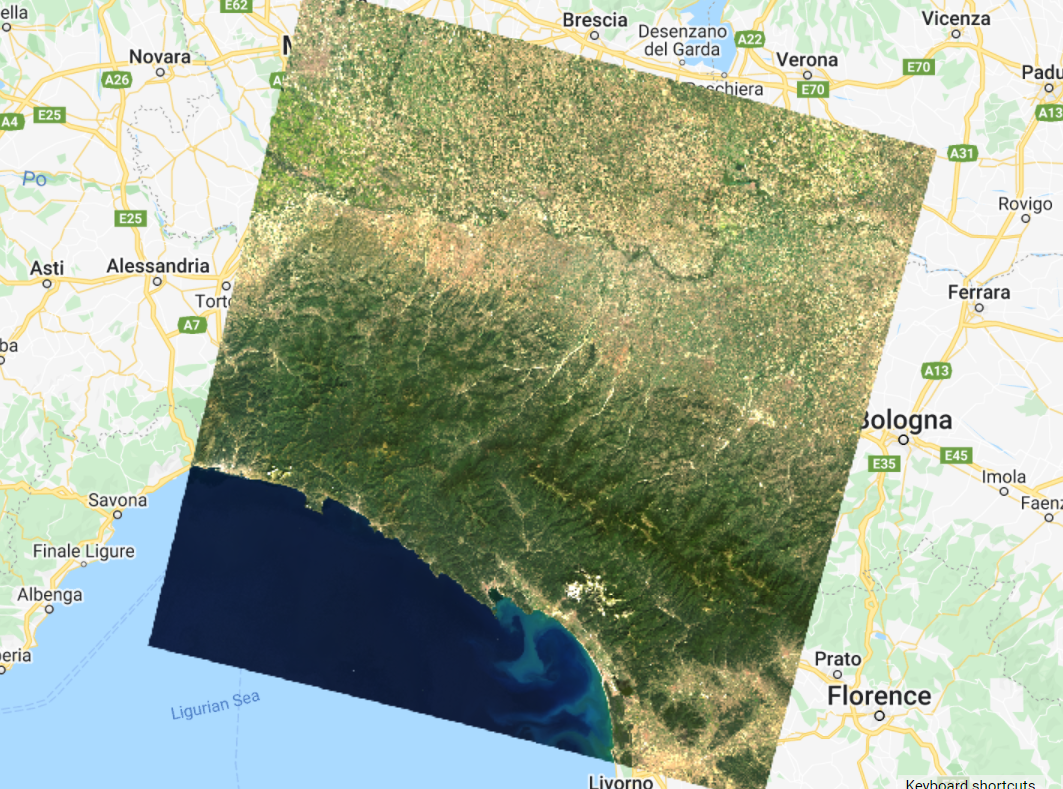
We will begin by creating training data manually, based on a clear Landsat image (Fig. F2.1.2). Copy the code block below to define your Landsat 8 scene variable and add it to the map. We will use a point in Milan, Italy, as the center of the area for our image classification.

Using the Geometry Tools, we will create points on the Landsat image that represent land cover classes of interest to use as our training data. We’ll need to do two things: (1) identify where each land cover occurs on the ground, and (2) label the points with the proper class number. For this exercise, we will use the classes and codes shown in Table 2.1.1.

Table 2.1.1 Land cover classes

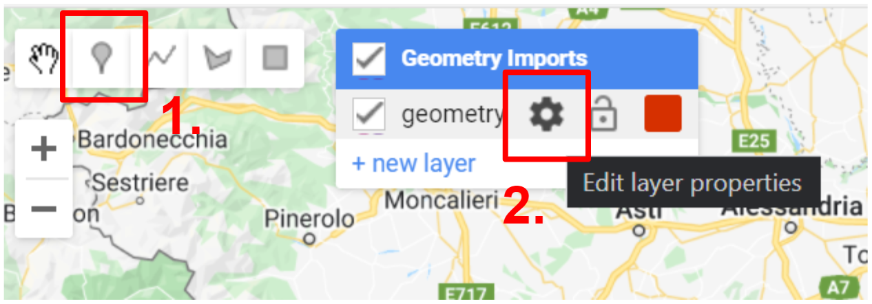
In the Geometry Tools, click on the marker option (Fig. F2.1.3). This will create a point geometry which will show up as an import named “geometry”. Click on the gear icon to configure this import.

We will start by collecting forest points, so name the import forest. Import it as a FeatureCollection, and then click + Property. Name the new property “class” and give it a value of 0 (Fig. F2.1.4). We can also choose a color to represent this class. For a forest class, it is natural to choose a green color. You can choose the color you prefer by clicking on it, or, for more control, you can use a hexadecimal value.

Hexadecimal values are used throughout the digital world to represent specific colors across computers and operating systems. They are specified by six values arranged in three pairs, with one pair each for the red, green, and blue brightness values. If you’re unfamiliar with hexadecimal values, imagine for a moment that colors were specified in pairs of base 10 numbers instead of pairs of base 16. In that case, a bright pure red value would be “990000”; a bright pure green value would be “009900”; and a bright pure blue value would be “000099”. A value like “501263” would be a mixture of the three colors, not especially bright, having roughly equal amounts of blue and red, and much less green: a color that would be a shade of purple. To create numbers in the hexadecimal system, which might feel entirely natural if humans had evolved to have 16 fingers, sixteen “digits” are needed: a base 16 counter goes 0, 1, 2, 3, 4, 5, 6, 7, 8, 9, A, B, C, D, E, F, then 10, 11, and so on. Given that counting framework, the number “FF” is like “99” in base 10: the largest two-digit number. The hexadecimal color used for coloring the letters of the word FeatureCollection in this book, a color with roughly equal amounts of blue and red, and much less green, is “7F1FA2”  

Returning to the coloring of the forest points, the hexadecimal value “589400” is a little bit of red, about twice as much green, and no blue: the deep green seen in Figure F2.1.4. Enter that value, with or without the “#” in front, and click OK after finishing the configuration.

Now, in the Geometry Imports, we will see that the import has been renamed forest. Click on it to activate the drawing mode (Fig. F2.1.5) in order to start collecting forest points.

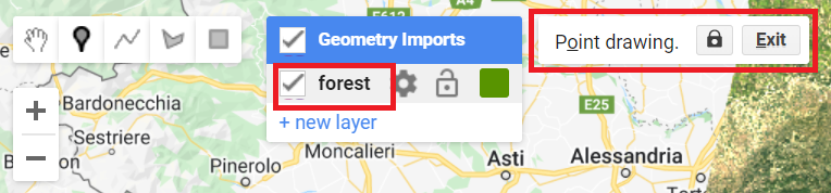
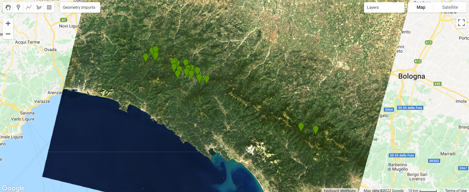
Now, start collecting points over forested areas (Fig. F2.1.6). Zoom in and out as needed. You can use the satellite basemap to assist you, but the basis of your collection should be the Landsat image. Remember that the more points you collect, the more the classifier will learn from the information you provide. For now, let’s set a goal to collect 25 points per class. Click Exit next to Point drawing (Fig. F2.1.5) when finished.

Repeat the same process for the other classes by creating new layers (Fig. F2.1.7). Don’t forget to import using the FeatureCollection option as mentioned above. For the developed class, collect points over urban areas. For the water class, collect points over the Ligurian Sea, and also look for other bodies of water, like rivers. For the herbaceous class, collect points over agricultural fields. Remember to set the “class” property for each class to its corresponding code (see Table 2.1.1) and click Exit once you finalize collecting points for each class as mentioned above. We will be using the following hexadecimal colors for the other classes: #FF0000 for developed, #1A11FF for water, and #D0741E for herbaceous. 

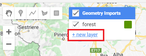
You should now have four FeatureCollection imports named forest, developed, water, and herbaceous (Fig. F2.1.8).

Code Checkpoint F21a. The book’s repository contains a script that shows what your code should look like at this point.

If you wish to have the exact same results demonstrated in this chapter from now on, continue beginning with this Code Checkpoint. If you use the points collected yourself, the results may vary from this point forward.

The next step is to combine all the training feature collections into one. Copy and paste the code below to combine them into one FeatureCollection called trainingFeatures. Here, we use the flatten method to avoid having a collection of feature collections—we want individual features within our FeatureCollection.

Note: Alternatively, you could use an existing set of reference data. For example, the European Space Agency (ESA) WorldCover dataset is a global map of land use and land cover derived from ESA’s Sentinel-2 imagery at 10 m resolution. With existing datasets, we can randomly place points on pixels classified as the classes of interest (if you are curious, you can explore the Earth Engine documentation to learn about the ee.Image.stratifiedSample and the ee.FeatureCollection.randomPoints methods). The drawback is that these global datasets will not always contain the specific classes of interest for your region, or may not be entirely accurate at the local scale. Another option is to use samples that were collected in the field (e.g., GPS points). In Chap. F5.0, you will see how to upload your own data as Earth Engine assets.

In the combined FeatureCollection, each Feature point should have a property called “class”. The class values are consecutive integers from 0 to 3 (you could verify that this is true by printing trainingFeatures and checking the properties of the features).

Now that we have our training points, copy and paste the code below to extract the band information for each class at each point location. First, we define the prediction bands to extract different spectral and thermal information from different bands for each class. Then, we use the sampleRegions method to sample the information from the Landsat image at each point location. This method requires information about the FeatureCollection (our reference points), the property to extract (“class”), and the pixel scale (in meters).

You can check whether the classifierTraining object extracted the properties of interest by printing it and expanding the first feature. You should see the band and class information (Fig. F2.1.9).

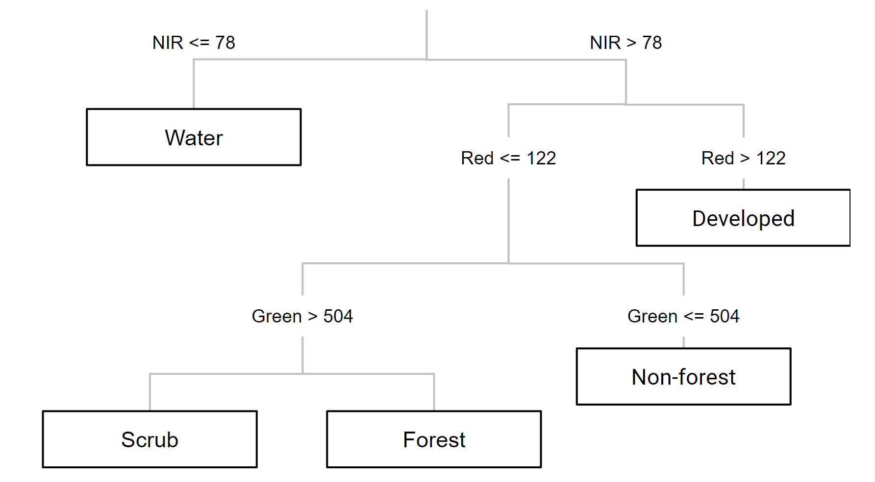
Now we can choose a classifier. The choice of classifier is not always obvious, and there are many options from which to pick—you can quickly expand the ee.Classifier object under Docs to get an idea of how many options we have for image classification. Therefore, we will be testing different classifiers and comparing their results. We will start with a Classification and Regression Tree (CART) classifier, a well-known classification algorithm (Fig. F2.1.10) that has been around for decades.

Copy and paste the code below to instantiate a CART classifier (ee.Classifier.smileCart) and train it.

Essentially, the classifier contains the mathematical rules that link labels to spectral information. If you print the variable classifier and expand its properties, you can confirm the basic characteristics of the object (bands, properties, and classifier being used). If you print classifier.explain, you can find a property called “tree” that contains the decision rules.

After training the classifier, copy and paste the code below to classify the Landsat image and add it to the Map.

Note that, in the visualization parameters, we define a palette parameter which in this case represents colors for each pixel value (0–3, our class codes). We use the same hexadecimal colors used when creating our training points for each class. This way, we can associate a color with a class when visualizing the classified image in the Map.

Inspect the result: Activate the Landsat composite layer and the satellite basemap to overlay with the classified images (Fig. F2.1.11). Change the layers’ transparency to inspect some areas. What do you notice? The result might not look very satisfactory in some areas (e.g., confusion between developed and herbaceous classes). Why do you think this is happening? There are a few options to handle misclassification errors:

• Collect more training data We can try incorporating more points to have a more representative sample of the classes.
• Tune the model Classifiers typically have “hyperparameters,” which are set to default values. In the case of classification trees, there are ways to tune the number of leaves in the tree, for example. Tuning models is addressed in Chap. F2.2.
• Try other classifiers If a classifier’s results are unsatisfying, we can try some of the other classifiers in Earth Engine to see if the result is better or different.
• Expand the collection location It is good practice to collect points across the entire image and not just focus on one location. Also, look for pixels of the same class that show variability (e.g., for the developed class, building rooftops look different than house rooftops; for the herbaceous class, crop fields show distinctive seasonality/phenology). 
• Add more predictors We can try adding spectral indices to the input variables; this way, we are feeding the classifier new, unique information about each class. For example, there is a good chance that a vegetation index specialized for detecting vegetation health (e.g., NDVI) would improve the developed versus herbaceous classification.

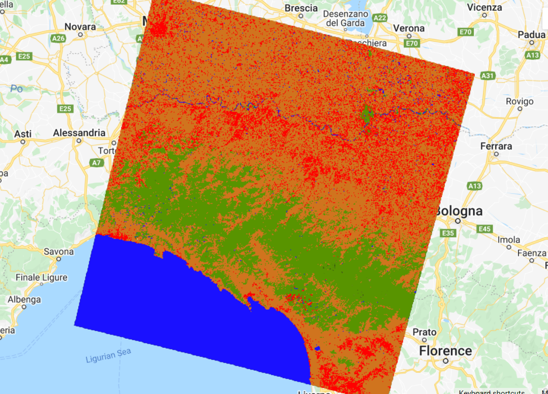
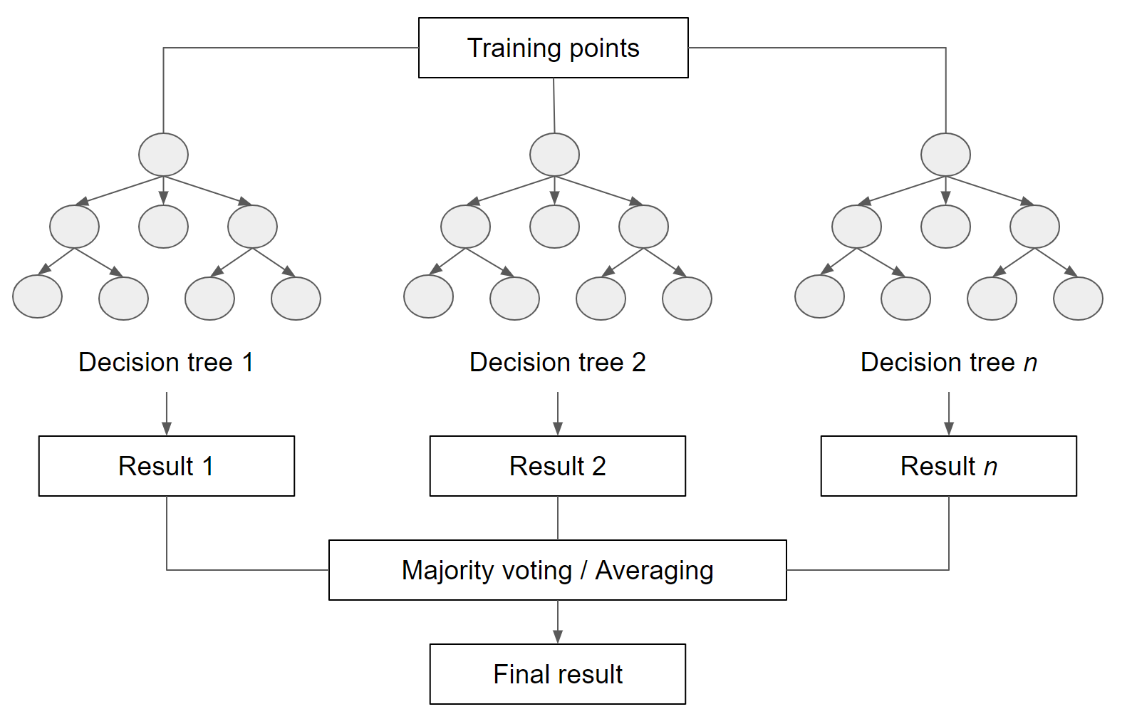
For now, we will try another supervised learning classifier that is widely used: Random Forests (RF). The RF algorithm (Breiman 2001, Pal 2005) builds on the concept of decision trees, but adds strategies to make them more powerful. It is called a “forest” because it operates by constructing a multitude of decision trees. As mentioned previously, a decision tree creates the rules which are used to make decisions. A Random Forest will randomly choose features and make observations, build a forest of decision trees, and then use the full set of trees to estimate the class. It is a great choice when you do not have a lot of insight about the training data.

Copy and paste the code below to train the RF classifier (ee.Classifier.smileRandomForest) and apply the classifier to the image. The RF algorithm requires, as its argument, the number of trees to build. We will use 50 trees.

Note that in the ee.Classifier.smileRandomForest documentation (Docs tab), there is a seed (random number) parameter. Setting a seed allows you to exactly replicate your model each time you run it. Any number is acceptable as a seed.

Inspect the result (Fig. F2.1.13). How does this classified image differ from the CART one? Is the classifications better or worse? Zoom in and out and change the transparency of layers as needed. In Chap. F2.2, you will see more systematic ways to assess what is better or worse, based on accuracy metrics.

Code Checkpoint F21b. The book’s repository contains a script that shows what your code should look like at this point.

Section 2. Unsupervised Classification

In an unsupervised classification, we have the opposite process of supervised classification. Spectral classes are grouped first and then categorized into clusters. Therefore, in Earth Engine, these classifiers are ee.Clusterer objects. They are “self-taught” algorithms that do not use a set of labeled training data (i.e., they are “unsupervised”). You can think of it as performing a task that you have not experienced before, starting by gathering as much information as possible. For example, imagine learning a new language without knowing the basic grammar, learning only by watching a TV series in that language, listening to examples, and finding patterns.

Similar to the supervised classification, unsupervised classification in Earth Engine has this workflow:

1. Assemble features with numeric properties in which to find clusters (training data).
2. Select and instantiate a clusterer.
3. Train the clusterer with the training data.
4. Apply the clusterer to the scene (classification).
5. Label the clusters.

In order to generate training data, we will use the sample method, which randomly takes samples from a region (unlike sampleRegions, which takes samples from predefined locations). We will use the image’s footprint as the region by calling the geometry method. Additionally, we will define the number of pixels (numPixels) to sample—in this case, 1000 pixels—and define a tileScale of 8 to avoid computation errors due to the size of the region. Copy and paste the code below to sample 1000 pixels from the Landsat image. You should add to the same script as before to compare supervised versus unsupervised classification results at the end.

Now we can instantiate a clusterer and train it. As with the supervised algorithms, there are many unsupervised algorithms to choose from. We will use the k-means clustering algorithm, which is a commonly used approach in remote sensing. This algorithm identifies groups of pixels near each other in the spectral space (image x bands) by using an iterative regrouping strategy. We define a number of clusters, k, and then the method randomly distributes that number of seed points into the spectral space. A large sample of pixels is then grouped into its closest seed, and the mean spectral value of this group is calculated. That mean value is akin to a center of mass of the points, and is known as the centroid. Each iteration recalculates the class means and reclassifies pixels with respect to the new means. This process is repeated until the centroids remain relatively stable and only a few pixels change from class to class on subsequent iterations.

Copy and paste the code below to request four clusters, the same number as for the supervised classification, in order to directly compare them.

Now copy and paste the code below to apply the clusterer to the image and add the resulting classification to the Map (Fig. F2.1.15). Note that we are using a method called randomVisualizer to assign colors for the visualization. We are not associating the unsupervised classes with the color palette we defined earlier in the supervised classification. Instead, we are assigning random colors to the classes, since we do not yet know which of the unsupervised classes best corresponds to each of the named classes (e.g., forest , herbaceous). Note that the colors in Fig. F1.2.15 might not be the same as you see on your Map, since they are assigned randomly.

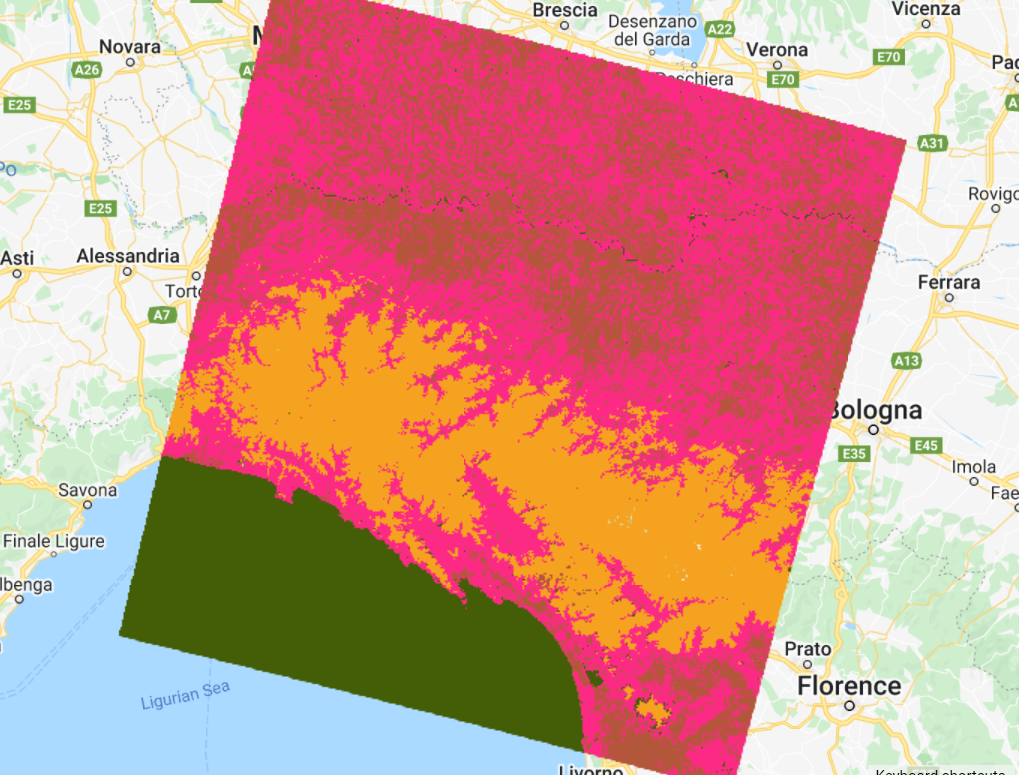
Inspect the results. How does this classification compare to the previous ones? If preferred, use the Inspector to check which classes were assigned to each pixel value (“cluster” band) and change the last line of your code to apply the same palette used for the supervised classification results (see Code Checkpoint below for an example).

Another key point of classification is the accuracy assessment of the results. This will be covered in Chap. F2.2.

Code Checkpoint F21c. The book’s repository contains a script that shows what your code should look like at this point.

Synthesis

Test if you can improve the classifications by completing the following assignments.

Assignment 1. For the supervised classification, try collecting more points for each class. The more points you have, the more spectrally represented the classes are. It is good practice to collect points across the entire composite and not just focus on one location. Also look for pixels of the same class that show variability. For example, for the water class, collect pixels in parts of rivers that vary in color. For the developed class, collect pixels from different rooftops.

Assignment 2. Add more predictors. Usually, the more spectral information you feed the classifier, the easier it is to separate classes. Try calculating and incorporating a band of  NDVI or the Normalized Difference Water Index (Chap. F2.0) as a predictor band. Does this help the classification? Check for developed areas that were being classified as herbaceous or vice versa.

Assignment 3. Use more trees in the Random Forest classifier. Do you see any improvements compared to 50 trees? Note that the more trees you have, the longer it will take to compute the results, and that more trees might not always mean better results.

Assignment 4. Increase the number of samples that are extracted from the composite in the unsupervised classification. Does that improve the result?

Assignment 5. Increase the number k of clusters for the k-means algorithm. What would happen if you tried 10 classes? Does the classified map result in meaningful classes?

Assignment 6. Test other clustering algorithms. We only used k-means; try other options under the ee.Clusterer object.

Conclusion

Classification algorithms are key for many different applications because they allow you to predict categorical variables. You should now understand the difference between supervised and unsupervised classification and have the basic knowledge on how to handle misclassifications. By being able to map the landscape for land use and land cover, we will also be able to monitor how it changes (Part F4).

Feedback

To review this chapter and make suggestions or note any problems, please go now to bit.ly/EEFA-review. You can find summary statistics from past reviews at bit.ly/EEFA-reviews-stats.

References

Cloud-Based Remote Sensing with Google Earth Engine. (n.d.). CLOUD-BASED REMOTE SENSING WITH GOOGLE EARTH ENGINE. https://www.eefabook.org/

Cloud-Based Remote Sensing with Google Earth Engine. (2024). In Springer eBooks. https://doi.org/10.1007/978-3-031-26588-4

Breiman L (2001) Random forests. Mach Learn 45:5–32. https://doi.org/10.1023/A:1010933404324

Gareth J, Witten D, Hastie T, Tibshirani R (2013) An Introduction to Statistical Learning. Springer

Géron A (2019) Hands-on Machine Learning with Scikit-Learn, Keras and TensorFlow: Concepts, Tools, and Techniques to Build Intelligent Systems. O’Reilly Media, Inc.

Goodfellow I, Bengio Y, Courville A (2016) Deep Learning. MIT Press

Hastie T, Tibshirani R, Friedman JH (2009) The Elements of Statistical Learning: Data Mining, Inference, and Prediction. Springer

Li M, Zang S, Zhang B, et al (2014) A review of remote sensing image classification techniques: The role of spatio-contextual information. Eur J Remote Sens 47:389–411. https://doi.org/10.5721/EuJRS20144723

Müller AC, Guido S (2016) Introduction to Machine Learning with Python: A Guide for Data Scientists. O’Reilly Media, Inc.

Pal M (2005) Random forest classifier for remote sensing classification. Int J Remote Sens 26:217–222. https://doi.org/10.1080/01431160412331269698

Witten IH, Frank E, Hall MA, et al (2005) Practical machine learning tools and techniques. In: Data Mining. pp 4