Cloud-Based Remote Sensing with Google Earth Engine

Fundamentals and Applications

Part F3: Advanced Image Processing
Once you understand the basics of processing images in Earth Engine, this Part will present some of the more advanced processing tools available for treating individual images. These include creating regressions among image bands, transforming images with pixel-based and neighborhood-based techniques, and grouping individual pixels into objects that can then be classified.
Chapter F3.3: Object-Based Image Analysis
Authors
Morgan A. Crowley, Jeffrey Cardille, Noel Gorelick
Overview
Pixel-based classification can include unwanted noise. Techniques for object-based image analysis are designed to detect objects within images, making classifications that can address this issue of classification noise. In this chapter, you will learn how region-growing can be used to identify objects in satellite imagery within Earth Engine. By understanding how objects can be delineated and treated in an image, students can apply this technique to their own images to produce landscape assessments with less extraneous noise. Here we treat images with an object delineator and view the results of simple classifications to view similarities and differences.
Learning Outcomes
- Learning about object-based image classification in Earth Engine.
- Controlling noise in images by adjusting different aspects of object segmentation.
- Understanding differences through time of noise in images.
- Creating and viewing objects from different sensors.
Assumes you know how to:
- Import images and image collections, filter, and visualize (Part F1).
- Perform basic image analysis: select bands, compute indices, create masks, classify images (Part F2).
- Create a function for code reuse (Chap. F1.0).
- Perform pixel-based supervised and unsupervised classification (Chap. F2.1).
Github Code link for all tutorials
This code base is collection of codes that are freely available from different authors for google earth engine.
Introduction to Theory
Building upon traditional pixel-based classification techniques, object-based image analysis classifies imagery into objects using perception-based, meaningful knowledge (Blaschke et al. 2000, Blaschke 2010, Weih and Riggan 2010). Detecting and classifying objects in a satellite image is a two-step approach. First, the image is segmented using a segmentation algorithm. Second, the landscape objects are classified using either supervised or unsupervised approaches. Segmentation algorithms create pixel clusters using imagery information such as texture, color or pixel values, shape, and size. Object-based image analysis is especially useful for mapping forest disturbances (Blaschke 2010, Wulder et al. 2004) because additional information and context are integrated into the classification through the segmentation process. One object-based image analysis approach available in Earth Engine is the Simple Non-Iterative Clustering (SNIC) segmentation algorithm (Achanta and Süsstrunk 2017). SNIC is a bottom-up, seed-based segmentation algorithm that assembles clusters from neighboring pixels based on parameters of compactness, connectivity, and neighborhood size. SNIC has been used in previous Earth Engine-based research for mapping land use and land cover (Shafizadeh-Moghadam et al. 2021, Tassi and Vizzari 2020), wetlands (Mahdianpari et al. 2018 and 2020, Amani et al. 2019), burned areas (Crowley et al. 2019), sustainable development goal indicators (Mariathasan et al. 2019), and ecosystem services (Verde et al. 2020).
Practicum
Section 1. Unsupervised Classification
If you have not already done so, be sure to add the book’s code repository to the Code Editor by entering https://code.earthengine.google.com/?accept_repo=projects/gee-edu/book into your browser. The book’s scripts will then be available in the script manager panel. If you have trouble finding the repo, you can visit this link for help.
In earlier chapters (see Chap. F2.1), you saw how to perform a supervised and unsupervised classification. In this lab, we will focus on object-based segmentation and unsupervised classifications—a clean and simple way to look at the spectral and spatial variability that is seen by a classification algorithm.
We’ll now build a script in several numbered sections, giving you a chance to see how it is constructed as well as to observe intermediate and contrasting results as you proceed. We’ll start by defining a function for taking an image and breaking it into a set of unsupervised classes. When called, this function will divide the image into a specified number of classes, without directly using any spatial characteristics of the image.
Paste the following block into a new script.
// 1.1 Unsupervised k-Means classification |
We’ll also need a function to normalize the band values to a common scale from 0 to 1. This will be most useful when we are creating objects. Additionally, we will need a function to add the mean to the band name. Paste the following functions into your code. Note that the code numbering skips intentionally from 1.2 to 1.4; we will add section 1.3 later.
// 1.2 Simple normalization by maxes function. |
We’ll create a section that defines variables that you will be able to adjust. One important adjustable parameter is the number of clusters for the clusterer to use. Add the following code beneath the function definitions.
//////////////////////////////////////////////////////////// |
The script will allow you to zoom to a specified area for better viewing and exists already in the code repository check points. Add this code below.
//////////////////////////////////////////////////////////// |
Now, with these functions, parameters, and flags in place, let’s define a new image and set image-specific values that will help analyze it. We’ll put this in a new section of the code that contains “if” statements for images from multiple sensors. We set up the code like this because we will use several images from different sensors in the following sections, therefore they are preloaded so all that you have to do is to change the parameter "whichImage". In this particular Sentinel-2 image, focus on differentiating forest and non-forest regions in the Puget Sound, Washington, USA. The script will automatically zoom to the region of interest.
////////////////////////////////////////////////////////// |
Now, let’s clip the image to the study area we are interested in, then extract the bands to use for the classification process.
//////////////////////////////////////////////////////////// |
Now, let’s view the per-pixel unsupervised classification, produced using the k-means classifier. Note that, as we did earlier, we skip a section of the code numbering (moving from section 4 to section 6), which we will fill in later as the script is developed further.
//////////////////////////////////////////////////////////// |
Then insert this code, so that you can zoom if requested.
//////////////////////////////////////////////////////////// |
Code Checkpoint F33a. The book’s repository contains a script that shows what your code should look like at this point.
Run the script. It will draw the study area in a true-color view (Fig. F3.3.1), where you can inspect the complexity of the landscape as it would have appeared to your eye in 2016, when the image was captured.
Fig. F3.3.1 True-color Sentinel-2 image from 2016 for the study area |

Note harvested forests of different ages, the spots in the northwest part of the study area that might be naturally treeless, and the straight easements for transmission lines in the easten part of the study area. You can switch Earth Engine to satellite view and change the transparency of the drawn layer to inspect what has changed in the years since the image was captured.
As it drew your true-color image, Earth Engine also executed the k-means classification and added it to your set of layers. Turn up the visibility of layer 6.1 Per-Pixel Unsupervised, which shows the four-class per-pixel classification result using randomly selected colors. The result should look something like Fig. F3.3.2.
Fig. F3.3.2 Pixel-based unsupervised classification using four-class k-means unsupervised classification using bands from the visible spectrum |

Take a look at the image that was produced, using the transparency slider to inspect how well you think the classification captured the variability in the landscape and classified similar classes together, then answer the following questions.
Question 1. In your opinion, what are some of the strengths and weaknesses of the map that resulted from your settings?
Question 2. Part of the image that appears to our eye to represent a single land use might be classified by the k-means classification as containing different clusters. Is that a problem? Why or why not?
Question 3. A given unsupervised class might represent more than one land use / land cover type in the image. Use the Inspector to find classes for which there were these types of overlaps. Is that a problem? Why or why not?
Question 4. You can change the numberOfUnsupervisedClusters variable to be more or less than the default value of 4. Which, if any, of the resulting maps produce a more satisfying image? Is there an upper limit at which it is hard for you to tell whether the classification was successful or not?
As discussed in earlier chapters, the visible part of the electromagnetic spectrum contains only part of the information that might be used for a classification. The short-wave infrared bands have been seen in many applications to be more informative than the true-color bands.
Return to your script and find the place where threeBandsToDraw is set. That variable is currently set to B4, B3, and B2. Comment out that line and use the one below, which will set the variable to B8, B11, and B12. Make the same change for the variable bandsToUse. Now run this modified script, which will use three new bands for the classification and also draw them to the screen for you to see. You’ll notice that this band combination provides different contrast among cover types. For example, you might now notice that there are small bodies of water and a river in the scene, details that are easy to overlook in a true-color image. With numberOfUnsupervisedClusters still set at 4, your resulting classification should look like Fig. F3.3.3.
Fig. F3.3.3 Pixel-based unsupervised classification using four-class k-means unsupervised classification using bands from outside of the visible spectrum |

Question 5. Did using the bands from outside the visible part of the spectrum change any classes so that they are more cleanly separated by land use or land cover? Keep in mind that the colors are randomly chosen in each of the images are unrelated—a class colored brown in Fig. F3.3.2 might well be pink in Fig. F3.3.3.
Question 6. Experiment with adjusting the numberOfUnsupervisedClusters with this new data set. Is one combination preferable to another, in your opinion? Keep in mind that there is no single answer about the usefulness of an unsupervised classification beyond asking whether it separates classes of importance to the user.
Code Checkpoint F33b. The book’s repository contains a script that shows what your code should look like at this point. In that code, the numberOfUnsupervisedClusters is set to 4, and the infrared bands are used as part of the classification process.
Section 2. Detecting Objects in Imagery with the SNIC Algorithm
The noise you noticed in the pixel-based classification will now be improved using a two-step approach for object-based image analysis. First, you will segment the image using the SNIC algorithm, and then you will classify it using a k-means unsupervised classifier. Return to your script, where we will add a new function. Noting that the code’s sections are numbered, find code section 1.2 and add the function below beneath it.
// 1.3 Seed Creation and SNIC segmentation Function |
As you see, the function assembles parameters needed for running SNIC (Achanta and Süsstrunk 2017, Crowley et al. 2019), the function that delineates objects in an image. A call to SNIC takes several parameters that we will explore. Add the following code below code section 2.2.
// 2.3 Object-growing parameters to change |
Now add a call to the SNIC function. You’ll notice that it takes the parameters specified in code section 2 and sends them to the SNIC algorithm. Place the code below into the script as the code’s section 5, between sections 4 and 6.
//////////////////////////////////////////////////////////// |
Now run the script. It will draw several layers, with the one shown in Fig. F3.3.4 on top.
Fig. F3.3.4 SNIC clusters, with randomly chosen colors for each cluster |
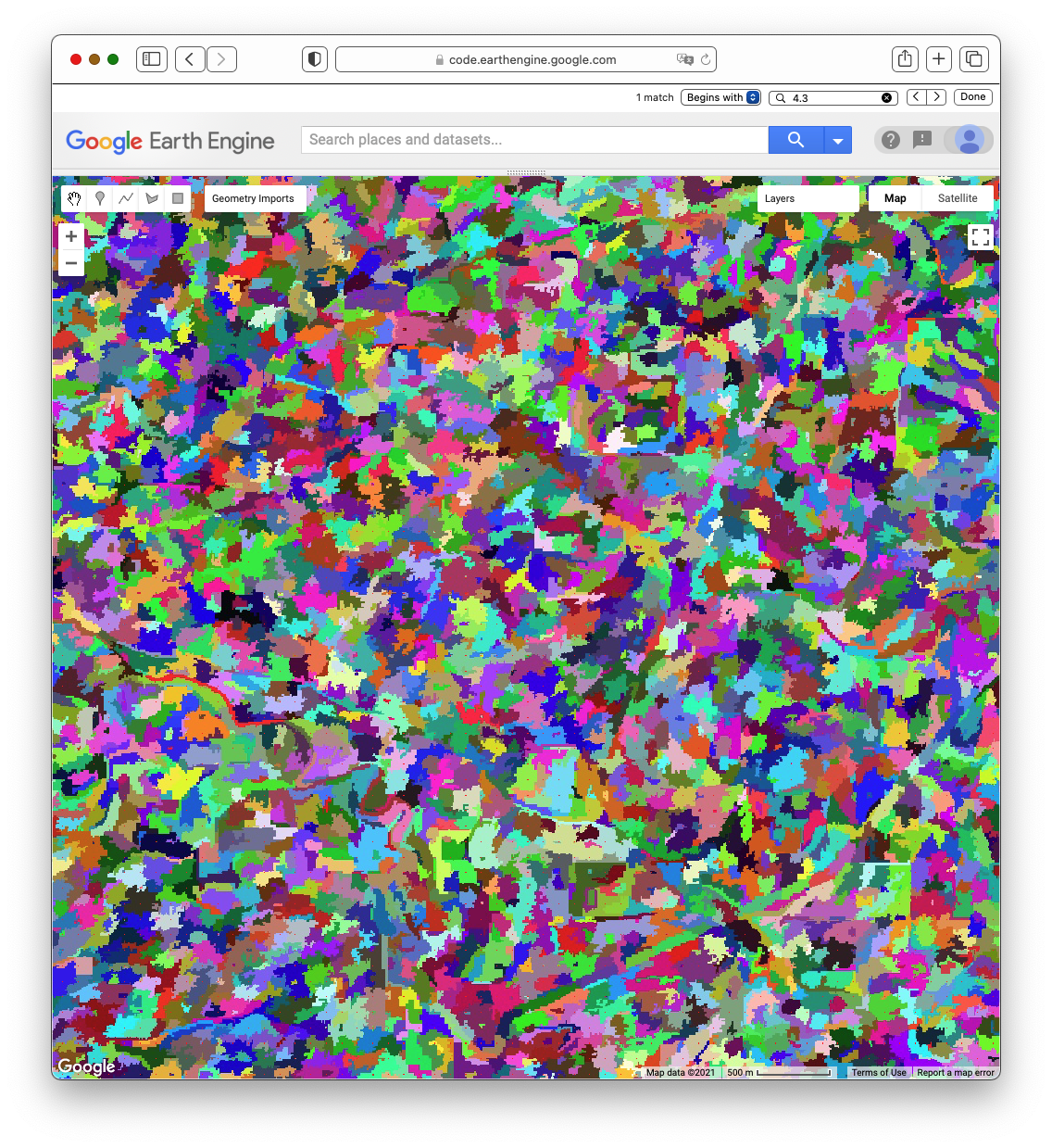
This shows the work of SNIC on the image sent to it—in this case, on the composite of bands 8, 11, and 12. If you look closely at the multicolored layer, you can see small red “seed” pixels. To initiate the process, these seeds are created and used to form square or hexagonal “super-pixels” at the spacing given by the parameters passed to the function. The edges of these blocks are then pushed and pulled, and directed to stop at edges in the input image. As part of the algorithm, some superpixels are then merged to form larger blocks, which is why you will find that some of the shapes contain two or more seed pixels.
Explore the structure by changing the transparency of layer 5 to judge how the image segmentation performs for the given set of parameter values. You can also compare layer 5.7 to layer 3.1. Layer 5.7 is a reinterpretation of layer 3.1 in which every pixel in a given shape of layer 5.3 is assigned the mean value of the pixels inside the shape. When parameterized in a way that is useful for a given project goal, parts of the image that are homogeneous will get the same color, while areas of high heterogeneity will get multiple colors.
Now spend some time exploring the effect of the parameters that control the code’s behavior. Use your tests to answer the questions below.
Question 7. What is the effect on the SNIC clusters of changing the parameter SNIC_SuperPixelSize?
Question 8. What is the effect of changing the parameter SNIC_Compactness?
Question 9. What are the effects of changing the parameters SNIC_Connectivity and SNIC_SeedShape?
Code Checkpoint F33c. The book’s repository contains a script that shows what your code should look like at this point.
Section 3. Object-Based Unsupervised Classification
The k-means classifier used in this tutorial is not aware that we would often prefer to have adjacent pixels be grouped into the same class—it has no sense of physical space. This is why you see the noise in the unsupervised classification. However, because we have re-colored the pixels in a SNIC cluster to all share the exact same band values, k-means will group all pixels of each cluster to have the same class. In the best-case scenario, this allows us to enhance our classification from being pixel-based to reveal clean and unambiguous objects in the landscape. In this section, we will classify these objects, exploring the strengths and limitations of finding objects in this image.
Return the SNIC settings to their first values, namely:
// The superpixel seed location spacing, in pixels. |
As code section 6.2, add this code, which will call the SNIC function and draw the results.
// 6.2 SNIC Unsupervised Classification for Comparison |
When you run the script, that new function will classify the image in layer 5.7, which is the recoloring of the original image according to the segments shown in layer 5. Compare the classification of the superpixels (6.3) with the unsupervised classification of the pixel-by-pixel values (6.1). You should be able to change the transparency of those two layers to compare them directly.
Question 10. What are the differences between the unsupervised classifications of the per-pixel and SNIC-interpreted images? Describe the tradeoff between removing noise and erasing important details.
Code Checkpoint F33d. The book’s repository contains a script that shows what your code should look like at this point.
Section 4. Classifications with More or Less Categorical Detail
Recall the variable numberOfUnsupervisedClusters, which directs the k-means algorithm to partition the data set into that number of classes. Because the colors are chosen randomly for layer 6.3, any change to this number typically results in an entirely different color scheme. Changes in the color scheme can also occur if you were to use a slightly different study area size between two runs. Although this can make it hard to compare the results of two unsupervised algorithms, it is a useful reminder that the unsupervised classification labels do not necessarily correspond to a single land use / land cover type.
Question 11. Find the numberOfUnsupervisedClusters variable in the code and set it to different values. You might test it across powers of two: 2, 4, 8, 16, 32, and 64 clusters will all look visually distinct. In your opinion, does one of them best discriminate between the classes in the image? Is there a particular number of colors that is too complicated for you to understand?
Question 12. What concrete criteria could you use to determine whether a particular unsupervised classification is good or bad for a given goal?
Section 5. Effects of SNIC Parameters
The number of classes controls the partition of the landscape for a given set of SNIC clusters. The four parameters of SNIC, in turn, influence the spatial characteristics of the clusters produced for the image. Adjust the four parameters of SNIC: SNIC_SuperPixelSize, SNIC_Compactness, SNIC_Connectivity, and SNIC_SeedShape. Although their workings can be complex, you should be able to learn what characteristics of the SNIC clustering they control by changing each one individually. At that point, you can explore the effects of changing multiple values for a single run. Recall that the ultimate goal of this workflow is to produce an unsupervised classification of landscape objects, which may relate to the SNIC parameters in very complex ways. You may want to start by focusing on the effect of the SNIC parameters on the cluster characteristics (layer 5.3), and then look at the associated unsupervised classification layer 6.
Question 13. What is the effect on the unsupervised classification of SNIC clusters of changing the parameter SNIC_SuperPixelSize?
Question 14. What is the effect of changing the parameter SNIC_Compactness?
Question 15. What are the effects of changing the parameters SNIC_Connectivity and SNIC_SeedShape?
Question 16. For this image, what is the combination of parameters that, in your subjective judgment, best captures the variability in the scene while minimizing unwanted noise?
Synthesis
Assignment 1. Additional images from other remote sensing platforms can be found in script F33s1 in the book's repository. Run the classification procedure on these images and compare the results from multiple parameter combinations.
Assignment 2. Although this exercise was designed to remove or minimize spatial noise, it does not treat temporal noise. With a careful choice of imagery, you can explore the stability of these methods and settings for images from different dates. Because the MODIS sensor, for example, can produce images on consecutive days, you would expect that the objects identified in a landscape would be nearly identical from one day to the next. Is this the case? To go deeper, you might contrast temporal stability as measured by different sensors. Are some sensors more stable in their object creation than others? To go even deeper, you might consider how you would quantify this stability using concrete measures that could be compared across different sensors, places, and times. What would these measures be?
Conclusion
Object-based image analysis is a method for classifying satellite imagery by segmenting neighboring pixels into objects using pre-segmented objects. The identification of candidate image objects is readily available in Earth Engine using the SNIC segmentation algorithm. In this chapter, you applied the SNIC segmentation and the unsupervised k-means algorithm to satellite imagery. You illustrated how the segmentation and classification parameters can be customized to meet your classification objective and to reduce classification noise. Now that you understand the basics of detecting and classifying image objects in Earth Engine, you can explore further by applying these methods on additional data sources.
Feedback
To review this chapter and make suggestions or note any problems, please go now to bit.ly/EEFA-review. You can find summary statistics from past reviews at bit.ly/EEFA-reviews-stats.
References
Cloud-Based Remote Sensing with Google Earth Engine. (n.d.). CLOUD-BASED REMOTE SENSING WITH GOOGLE EARTH ENGINE. https://www.eefabook.org/
Cloud-Based Remote Sensing with Google Earth Engine. (2024). In Springer eBooks. https://doi.org/10.1007/978-3-031-26588-4
Achanta R, Süsstrunk S (2017) Superpixels and polygons using simple non-iterative clustering. In: Proceedings - 30th IEEE Conference on Computer Vision and Pattern Recognition, CVPR 2017. pp 4895–4904
Amani M, Mahdavi S, Afshar M, et al (2019) Canadian wetland inventory using Google Earth Engine: The first map and preliminary results. Remote Sens 11:842. https://doi.org/10.3390/RS11070842
Blaschke T (2010) Object based image analysis for remote sensing. ISPRS J Photogramm Remote Sens 65:2–16. https://doi.org/10.1016/j.isprsjprs.2009.06.004
Blaschke T, Lang S, Lorup E, et al (2000) Object-oriented image processing in an integrated GIS/remote sensing environment and perspectives for environmental applications. Environ Inf planning, Polit public 2:555–570
Crowley MA, Cardille JA, White JC, Wulder MA (2019) Generating intra-year metrics of wildfire progression using multiple open-access satellite data streams. Remote Sens Environ 232:111295. https://doi.org/10.1016/j.rse.2019.111295
Mahdianpari M, Salehi B, Mohammadimanesh F, et al (2020) Big data for a big country: The first generation of Canadian wetland inventory map at a spatial resolution of 10-m using Sentinel-1 and Sentinel-2 data on the Google Earth Engine cloud computing platform. Can J Remote Sens 46:15–33. https://doi.org/10.1080/07038992.2019.1711366
Mahdianpari M, Salehi B, Mohammadimanesh F, et al (2019) The first wetland inventory map of Newfoundland at a spatial resolution of 10 m using Sentinel-1 and Sentinel-2 data on the Google Earth Engine cloud computing platform. Remote Sens 11:43 https://doi.org/10.3390/rs11010043
Mariathasan V, Bezuidenhoudt E, Olympio KR (2019) Evaluation of Earth observation solutions for Namibia’s SDG monitoring system. Remote Sens 11:1612. https://doi.org/10.3390/rs11131612
Shafizadeh-Moghadam H, Khazaei M, Alavipanah SK, Weng Q (2021) Google Earth Engine for large-scale land use and land cover mapping: An object-based classification approach using spectral, textural and topographical factors. GIScience Remote Sens 58:914–928. https://doi.org/10.1080/15481603.2021.1947623
Tassi A, Vizzari M (2020) Object-oriented LULC classification in Google Earth Engine combining SNIC, GLCM, and machine learning algorithms. Remote Sens 12:1–17. https://doi.org/10.3390/rs12223776
Verde N, Kokkoris IP, Georgiadis C, et al (2020) National scale land cover classification for ecosystem services mapping and assessment, using multitemporal Copernicus EO data and Google Earth Engine. Remote Sens 12:1–24. https://doi.org/10.3390/rs12203303Weih RC, Riggan ND (2010) Object-based classification vs. pixel-based classification: Comparative importance of multi-resolution imagery. Int Arch Photogramm Remote Sens Spat Inf Sci 38:C7
Wulder MA, Skakun RS, Kurz WA, White JC (2004) Estimating time since forest harvest using segmented Landsat ETM+ imagery. Remote Sens Environ 93:179–187. https://doi.org/10.1016/j.rse.2004.07.009