Cloud-Based Remote Sensing with Google Earth Engine
Fundamentals and Applications

Part A3: Terrestrial Applications
Earth’s terrestrial surface is analyzed regularly by satellites, in search of both change and stability. These are of great interest to a wide cross-section of Earth Engine users, and projects across large areas illustrate both the challenges and opportunities for life on Earth. Chapters in this Part illustrate the use of Earth Engine for disturbance, understanding long-term changes of rangelands, and creating optimum study sites.
Chapter A3.4: Forest Degradation and
Deforestation
Authors
Carlos Souza Jr., Karis Tenneson, John Dilger, Crystal Wespestad, Eric Bullock
Overview
Tropical forests are being disturbed by deforestation and forest degradation at an unprecedented pace (Hansen et al. 2013, Bullock et al. 2020). Deforestation completely removes the original forest cover and replaces it with another land cover type, such as pasture or agriculture fields. Generally speaking, forest degradation is a temporary or permanent disturbance, often caused by predatory logging, fires, or forest fragmentation, where the tree loss does not entirely change the land cover type. Forest degradation leads to a more complex environment with a mixture of vegetation, soil, tree trunks and branches, and fire ash. Defining a boundary between deforestation and forest degradation is not straightforward; at the time this chapter was written, there was no universally accepted definition for forest degradation (Aryal et al. 2021). Furthermore, the signal of forest degradation often disappears within one to two years, making degraded forests spectrally similar to undisturbed forests. Due to these factors, detecting and mapping forest degradation with remotely sensed optical data is more challenging than mapping deforestation.
The purpose of this chapter is to present a spectral unmixing algorithm and the Normalized Difference Fraction Index (NDFI) to detect and map both forest degradation and deforestation in tropical forests. This spectral unmixing model uses a set of generic endmembers (Souza et al. 2005a) to process any Landsat Surface Reflectance (Tier 1) scene available in Google Earth Engine. We present two examples of change detection applications, one comparing a pair of images acquired at different times a year apart by making a temporal color composite and an empirically defined change threshold, and another using a more extensive and dense time series approach.
Learning Outcomes
- Calculating NDFI, the Normalized Difference Fraction Index
- Interpreting fraction images and NDFI using a temporal color composite.
- Analyzing deforestation and forest degradation with NDFI
- Running a time-series change detection to detect forest change.
Helps if you know how to:
- Import images and image collections, filter, and visualize (Part F1).
- Perform basic image analysis: select bands, compute indices, create masks (Part F2).
- Use drawing tools to create points, lines, and polygons (Chap. F2.1).
- Run and interpret spectral unmixing models (Chap. F3.1).
- Use expressions to perform calculations on image bands (Chap. F3.1).
- Aggregate data to build a time series (Chap. F4.2).
- Perform a two-period change detection (Chap. F4.4).
Github Code link for all tutorials
This code base is collection of codes that are freely available from different authors for google earth engine.
Introduction to Theory
Landsat imagery has been extensively used to monitor deforestation (Woodcock et al. 2020). However, detecting and mapping forest degradation associated with selective logging is more elaborate and challenging. First efforts involved the application of spectral and textural indices to enhance the detection of canopy damage created by logging (Asner et al. 2002, Souza et al. 2005a), but these turned out to be more helpful in enhancing logging infrastructure using Landsat shortwave infrared bands (i.e., roads and log landings; Matricardi et al. 2007).
Alternatively, spectral mixture analysis (SMA) has been proposed to overcome the challenge of using whole-pixel information to detect and classify forest degradation. Landsat pixels typically contain a mixture of land cover components (Adams et al. 1995). The SMA method is based on the linear spectral unmixing model, as described in Chap. F3.1. The identification of the nature and number of pure spectra (often referred to in this context as “endmembers”) in the image scene is an important step in obtaining correct SMA models. In logged forests (and also in burned forest and forest edges), mixed pixels predominate and are expected to have a combination of green vegetation (GV), soil, non-photosynthetic vegetation (NPV), and shade-covered materials. Therefore, fraction images derived from SMA analyses are more suitable to enhance the detectability of logging infrastructure and canopy damage within degraded forests. For example, soil fractions reveal log landings and logging roads (Souza and Barreto 2000), while the NPV highlights forest canopy damage (Cochrane and Souza 1998, Souza et al. 2003), and the areas decreasing in GV indicate forest canopy gaps (Asner et al. 2004).
A study has shown that it is possible to generalize the SMA model to Landsat sensors (including TM, ETM+, and OLI) (Small 2004). Souza et al. (2005a) expanded the generalized SMA to handle five endmembers—GV, NPV, Soil, Shade, and Cloud —expected within forest degradation areas and proposed a novel compositional index based on SMA fractions, the Normalized Difference Fraction Index (NDFI).
The NDFI is computed as:
 (A3.4.1)
where  is the shade-normalized GV fraction given by,
 (A3.4.2)
NDFI values range from −1 to 1. For intact forests, NDFI shows high values (i.e., about 1) due to the combination of high GVshade (i.e., high GV and canopy Shade) and low NPV and Soil values. The NPV and Soil fractions increase as forests are more degraded, lowering NDFI values relative to the intact forests. Deforested areas exhibit very low GV and Shade and high NPV and Soil, making it possible to distinguish them from degraded forests based on NDFI magnitude.
Recent studies compared NDFI with other spectral indices. NDFI generated more accurate results in deforestation detection (Schultz et al. 2016) and forest degradation (Bullock et al. 2018) in time-series analysis. One of the key components for its success is lowering unwanted noise and accounting for illumination variability through the shade normalization applied to the GV fraction.
Practicum
Section 1. Spectral Mixture Analysis Model
Let us first define the Landsat endmembers based on Souza et al. (2005a). These endmembers were developed and tested in the Amazon. These endmembers work well in many other environments (see example applications for calculating NDFI in non-Amazonian tropical forest in Schultz et al. 2016 [Ethiopia and Viet Nam], Kusbach et al. 2017 [central Europe], and Hirschmugl et al. 2013 [Cameroon and Central African Republic]). If you are working in a different region, assess how well they perform for your forest types. The ratio of these endmembers that makes up the spectral signature of each pixel gives a good indication of the plant health and composition for that area. When the ratio shifts over time towards one or more of the endmembers we can quantify how the landscape is changing.
Below, we will create a new variable endmembers by copying the values from the code block below. The six numbers in square brackets define the pure reflectance values for the blue, green, red, SWIR1, and SWIR2 bands for each endmember material.
// SMA Model - Section 1 |
We will choose a single Landsat 5 image to work with for now, and select the bands we will need for the SMA and NDFI calculation.
Create a new variable image and assign it to the Landsat 5 image from the code block below. Select the visible, near infrared, and shortwave infrared bands. Then, center the map around the Landsat 5 image with a zoom scale of 10.
// Select a Landsat 5 scene on which to apply the SMA model. |
Next, we will need to create a couple of functions to use the endmembers and create the NDFI image. We will need to unmix the input Landsat image.
First, we will create a new function getSMAFractions that takes two parameters: image and endmembers. To unmix the image, we first select the visible, near-infrared, and short wave infrared bands, and call the unmix function with the endmembers used as the argument. Note: The order in which the bands are selected matters. For each endmember (GV, NPV, Soil, and Cloud) each value in the array represents the pure value for each band being passed in. For example, if the selected bands were ['SR_B2', 'SR_B3', 'SR_B4', 'SR_B5', 'SR_B6', 'SR_B7'] then the selected endmembers at position 0 would be:
- ‘SR_B2’ GV: 119
- ‘SR_B2’ NPV: 1514
- ‘SR_B2’ Soil: 1799
- ‘SR_B2’ Cloud: 4031
// Unmixing image using Singular Value Decomposition. |
We will now write the function to calculate NDFI. We could write it out line by line for each time we want to perform SMA or calculate NDFI. But having the equation implemented as a function gives us many benefits, including reducing redundancy, allowing us to map the function over a collection of images, and reducing errors from typos or other little bugs that can find their way into our code.
We will use the fraction images obtained with the getSMAFractions function above to calculate Shade, GVs, and NDFI using image expressions. This procedure will return a multiband image with the Shade, GVs, and NDFI bands added to the input image.
First, we will create a new variable sma and pass in the image and endmembers as arguments. Then calculate the Shade and GV shade-normalized (GVs) fractions from the SMA bands, and add the Shade and GVs bands to the SMA image. We calculate NDFI using an expression implementing Eq. A3.4.1, and add the new band to the SMA image.
// Calculate GVS and NDFI and add them to image fractions. |
We will use a color palette that spans from white, to pink (i.e., bare land), to yellow, to green to visualize the NDFI image. Higher values of NDFI will be green, while lower values will span the colors of white, pink, and yellow. Copy the code block below into your Code Editor.
// Define NDFI color table. |
Next, we can visualize all the hard work we have done unmixing each endmember and the NDFI bands (Fig. A3.4.1).
Create an image visualization object with bands 5, 4, and 3, chosen for visualization along with a min and max. Add the Landsat 5 image to the map using the image visualization object.
Now add each of the SMA bands and the NDFI band to the map. Note: Rather than defining the min, max, and bands for each of these in separate variables, we can pass in the object directly to the Map.addLayer function.
var imageVis={ |
a) b) c) d) e) |
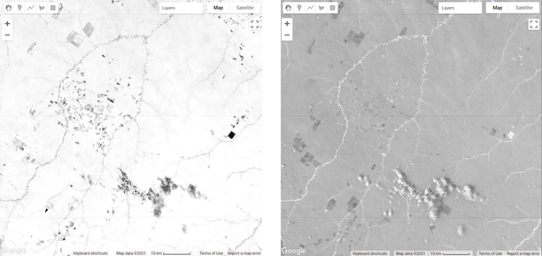
Fig. A3.4.1 Example maps of a) green vegetation shade normalized fraction (more vegetation is whiter); b) shade fraction (more shade is whiter); c) non-photosynthetic vegetation fraction (more NPV is whiter); d) green vegetation fraction (more vegetation is whiter); e) soil fraction (more soil is whiter). |
The last thing we will do in this section is to create a water and cloud mask. Water and clouds will have lower NDFI values. While water may not be too much of an issue, clouds will impact how we monitor forest degradation and loss, and thus we can simply mask them out. We can mask them using a thresholding method based on the values of our fraction images.
First, create a new function variable getWaterMask that takes an SMA image as the only argument.
Next, create a water mask using threshold values for the Shade, GV, and Soil bands, where Shade is greater than or equal to 0.65; GV is less than or equal to 0.15; and Soil is less than or equal to 0.05.
Now create a cloud mask by applying a threshold of 0.1 or greater to the Cloud band.
var getWaterMask=function(sma){ |
Next, we will combine the cloud and water masks using the max reducer. Since we want to mask both water and clouds, using the max works quite nicely here—as opposed to adding the images together—so we do not need to worry about overlaps.
Now add the cloud and water mask as a layer to the map.
Apply the cloud and water mask to the NDFI band using the updateMask function and invert the mask using the not function. Note: updateMask considers zeroes as invalid (i.e., to be masked) and ones as valid (i.e., to be kept). Since our original mask had values of 1 for cloud and water, we use the not function to invert the values.
var cloudWaterMask=cloud.max(water); |
Code Checkpoint A34a. The book’s repository contains a script that shows what your code should look like at this point.
Section 2. Deforestation and Forest Degradation Change Detection
To observe changes in the landscape over time, you need to create an NDFI image for two points in time and then calculate the difference between them. Previous studies have shown that images should not be more than one year apart because the forest degradation disturbance quickly disappears with tree foliage and understory vegetation growth. Changes in NDFI are a good indicator of forest change.
Now we will start using the functions we have built. First, we perform the SMA on a Landsat 5 image. Recall that the SMA function wants only the visible, near-infrared, and shortwave infrared bands. When using Landsat 5, those correspond to bands 1–5 and band 7.
First, create a variable for the Landsat 5 scene specified in the code block below and select the visible, near-infrared, and shortwave infrared bands. Use the getSMAFractions function with the Landsat image and the endmembers. Rename the output SMA bands as GV, NPV, Soil, and Cloud.
// Select two Landsat 5 scenes on which to apply the SMA model. |
Before we move on to calculate the NDFI, we will add the previous Landsat scene and the fractional images to the map to inspect them (example results in Fig. A3.4.2).
// Center the image object. |
a) b) c) d) |
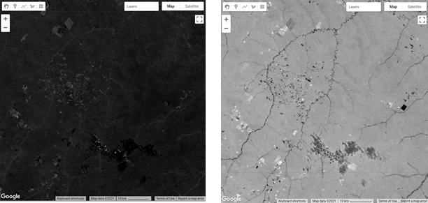
Fig. A3.4.2 Example maps of a) RGB composite of bands 5-4-3 (green is vegetation and brown is barren ground); b) soil fraction (more soil is whiter); c) green vegetation fraction (more vegetation is whiter), d) non-photosynthetic vegetation fraction (more NPV is whiter). |

Next, let’s set up a function to systematically reproduce the work we did computing NDFI, since we will need it a couple more times. Hereafter, we will be able to call that function instead of needing to explicitly write out each step, thus simplifying our code and making it easier to change if we need to later.
function getNDFI(smaImage){ |
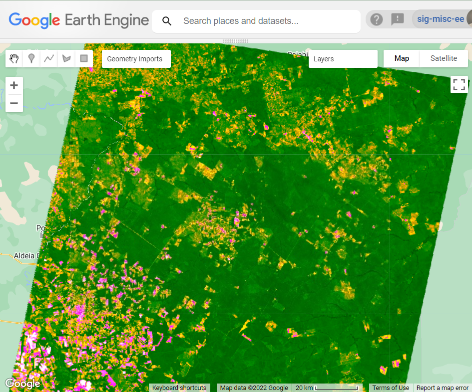
Then, calculate NDFI for the earlier Landsat image’s SMA bands (use smaTime0 as an input), using the getNDFI function you wrote. Add this NDFI image to the map displayed in the ndfiColors palette (Fig. A3.4.3). This will serve as your calculated NDFI for your earlier point in time, the pre-change time (this time was defined as imageTime0).
// Create the initial NDFI image and add it to the map. |
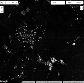
Fig. A3.4.3 NDFI image for the previous year obtained from the Landsat 5 (path/row 226/068) scene acquired on May 9, 2000. Orange colors indicate signs of forest disturbance associated with fires and selective logging. Pink and white colors are dry vegetation and bare soil in old deforested areas. Orange colors in pasturelands mean dry vegetation. |
Next, you will repeat this procedure to calculate the SMA fractions and NDFI of the second Landsat 5 image (smaTime1). You will utilize the same SMA method.
First, create a new variable (imageTime1), using the Landsat 5 scene from the code block below. Note that the band numbers for Landsat 8 are different from those for Landsat 5. In general, you should always make sure to check band names when working with multiple Landsat collections. Then, you will calculate the SMA fractions. The getSMAFractions function will rename the outputs to “GV”, “NPV”, “Soil”, and “Cloud”. Then, you will calculate NDFI for the new scene. Add an RGB composite and the NDFI to the map.
// Select a second Landsat 5 scene on which to apply the SMA model. |
Before looking at changes between the two NDFI images, use the opacity slider in the Layers panel of the map to manually view the differences between the NDFI outputs, and then the RGB outputs. Where do you expect to see the greatest changes between the two?
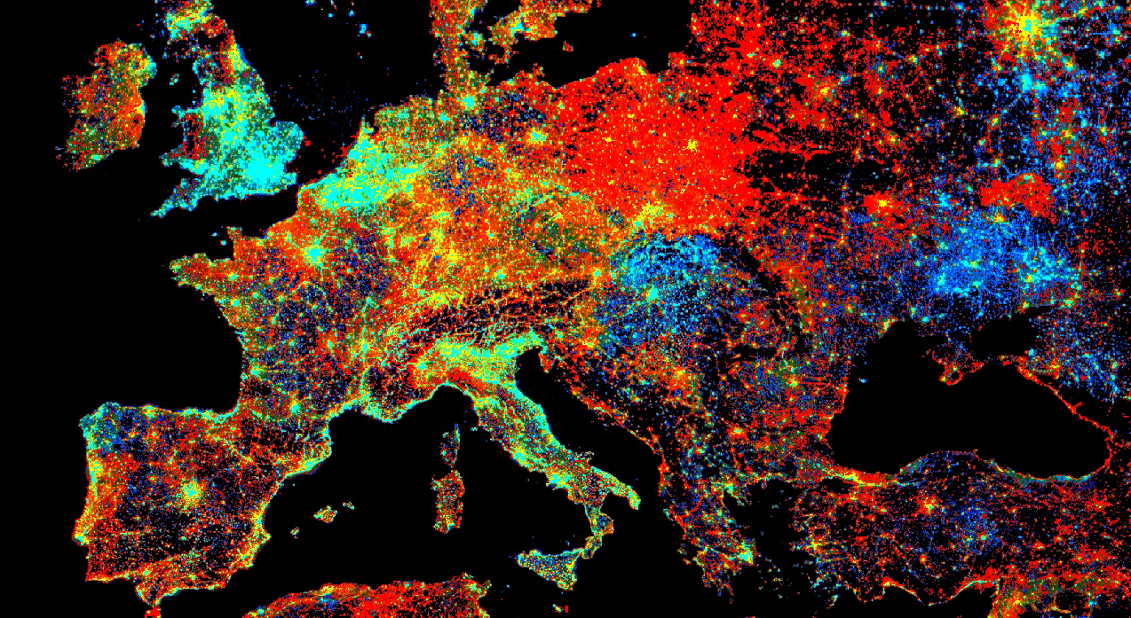
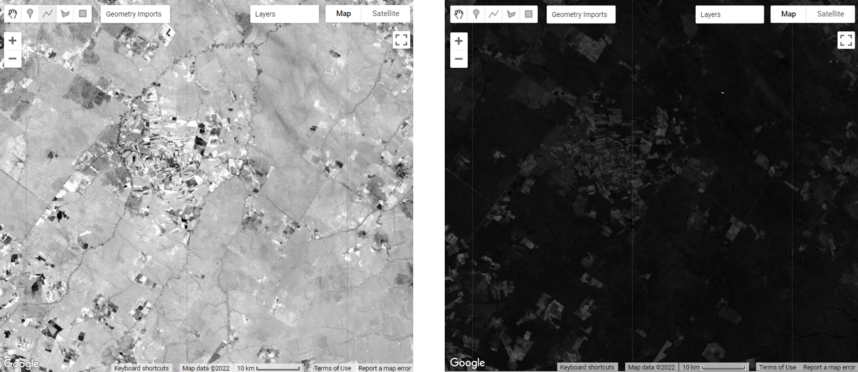
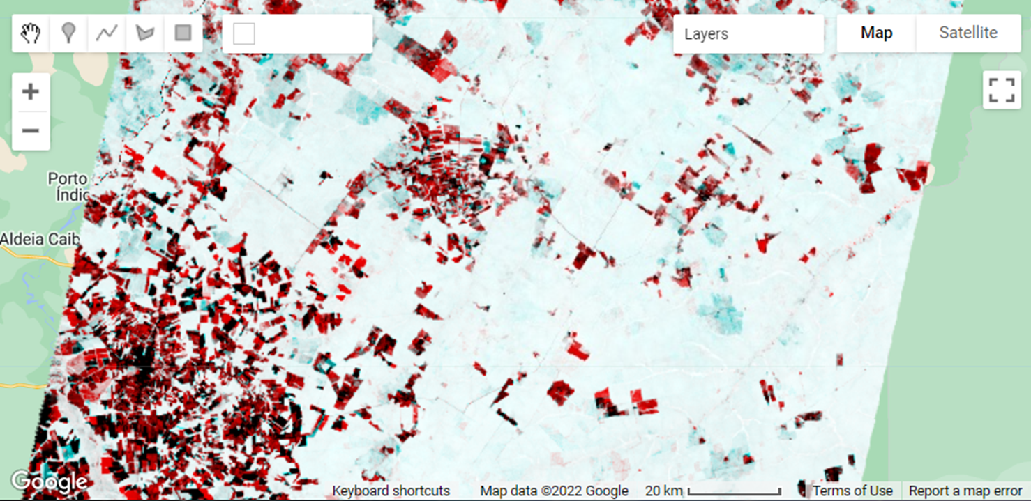
An easier way to enhance changes using a pair of images is to build a temporal color composite. To construct a temporal color composite, we add the first image date to the R color channel and the second to the G and B channels. An example of RGB color composite (as first described in Chap. F1.1) is shown in Fig. A3.4.4, using the NDFI_t0 (R) and NDFI_t1 (G and B). Deforestation appears in bright red colors since we assigned the first NDFI image to the R color channel, indicating forest in the previous year, and removal in the following (i.e., G and B colors have low NDFI values due to forest removal). In contrast, the cyan colors in the NDFI temporal color composite indicate vegetation regrowth in the second year. The gradient of dark to gray colors suggests no change in NDFI between the two dates.
a) b) c) d) |
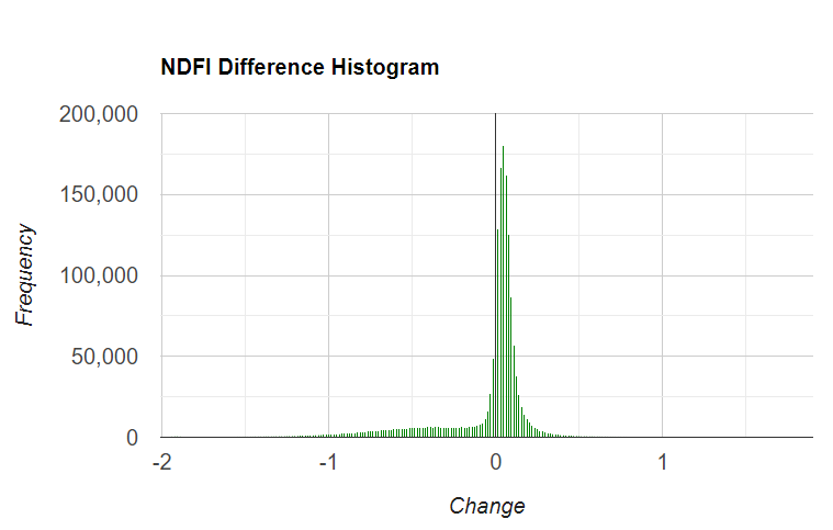
Fig. A3.4.4 Example of NDFI obtained for the first (a) and second (b) Landsat images, and a visualization of them using a temporal RGB color composite (c). Intense red colors are newly deforested areas, and light red are selectively logged forests. Cyan colors indicate vegetation regrowth in areas that were logged or burned a year ago or more. Example of NDFI difference histogram (d), with positive values indicating an increase in NDFI over time and negative values a decrease. Values at zero suggest no change. |


To find the change between our images, a simple difference method can be applied by subtracting the previous image from the current image. Then, we can apply an empirically defined threshold to classify the changes based on the inspection of the histogram and the NDFI temporal color composite. For more information on two-date differencing, see Chap. F4.4.
Next, we will combine the two NDFI images for time t0 and t1. Create a new variable ndfiChange and subtract the current NDFI image (made using Landsat 5 imagery from 2001) from the previous NDFI image (made using Landsat 5 imagery from 2000). Note: The NDFI is calculated using the image expression method applied to the SMA fraction presented in the code above. We then combine the two NDFI bands from 2000 and 2001 in one variable to display the change over time.
// Combine the two NDFI images in a single variable. |
Using the polygon drawing tool (as described in Chap. F2.1), draw a region that covers most of the ndfiChange image and rename it region in the variable import panel.
Next, make a histogram named histNDFIChange that bins the ndfiChange image using the region you just drew, and prints it to the Console. Optionally, click Run to view the histogram and identify some potential change thresholds. In your case the histogram may look slightly different.
var options={ |
Classify the difference image into new deforestation (red), forest degradation (orange), regrowth (cyan), and forest (green). The classification is based on slicing the NDFI difference image. Old deforested areas are detected using the NDFI first image date (t0).
Add the change classification and difference images to the map and click Run.
// Classify the NDFI difference image based on thresholds |
Finally, add code to add all the new layers to the map and click Run.
// Add layers to map |
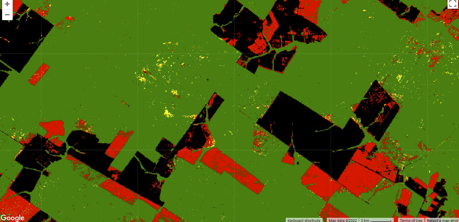
Fig. A3.4.5 shows an example of forest changes between two dates displayed using the cutoffs defined by the histogram. Categorizing the whole map into a simple system of no change, old deforestation, new deforestation, partial forest disturbance, and regrowth makes the forest use patterns in the region clearer. However, you must be careful with the thresholds you chose from the histogram when creating and interpreting the NDFI changes in this way, as those values can drastically alter your map. Consider when it might be more appropriate to use an RGB temporal color composite, and in what situations the classified map using the empirically defined thresholds would be better.
Fig. A3.4.5 Example of the change detection using two NDFI images. Green is remaining forest; black is old deforestation as detected in the first NDFI image; red highlights new deforestation; orange shows forest disturbance by logging or fires; and cyan is vegetation regrowth of forest since the previous date. |
Code Checkpoint A34b. The book’s repository contains a script that shows what your code should look like at this point.
Save your script for your own future use, as outlined in Chap. F1.0. Then, refresh the page to begin with a new script for the next section.
Section 3: Deforestation and Forest Degradation Time Series Analysis
To assess deforestation and forest degradation with a time series, we can use a Google Earth Engine tool called CODED (Bullock et al. 2018, Bullock et al. 2020). The algorithm is based on previous work in continuous land cover monitoring (Zhu and Woodcock 2014) and NDFI-based degradation mapping using spectral unmixing models (Souza et al. 2003 and 2005a). CODED has both a user-interface application and an API, which can be accessed in the Earth Engine Code Editor. For this lesson we will use the API.
Code Checkpoint A34c. The book’s repository contains a script to use to begin this section. You will need to start with that script and script and paste code below into it. The checkpoint accesses the modules of the CODED API and support functions. Note: importing large modules can cause your browser to hang for a moment while they load.
Detecting degraded forest regions requires knowledge of the characteristics of the forest of interest when it is in its normal healthy state. Higher NDFI values, near 1, typically indicate a healthy forest, but the magnitude range of NDFI for a healthy forest is dependent on forest density, type of forest ecosystem, and the seasonality of the area. Therefore, CODED uses a training period to find the typical values of NDFI generally seen in each forest over time. For each pixel, a regression model, similar to what was first presented in Chap. F4.6, is fit for NDFI values within the training period. The regression model is composed of a constant for overall NDFI magnitude, a sine and cosine term encapsulating seasonal and intra-annual variability, and an RMSE to account for noise. In this way, CODED can find typical temporal patterns in the landscape, account for clouds and sensor noise, and better distinguish forests from non-forested areas.
The code below sets up the study area, accesses the Landsat collection to be used, and defines the study period. For this example, we will use the geometry of the previous Landsat scene as our study area. Then, we define a new variable studyArea and assign it to the image we used when first exploring NDFI, retrieving its geometry using the geometry method. Then, we use the utils module to call the Inputs.getLandsat function, which accesses the ImageCollection. We then filter the images to a start date and end date of interest.. Note: CODED calibrates to find the typical variations in NDFI for the region by observing the NDFI patterns over time, so it is a good idea to filter the Landsat data so you have an extra six months to a year of data before the time period in which you are truly interested. For example, if you wanted to study forest change from 2000–2010, it would be good practice to use 1999 as the start date and 2010 as the end date.. Paste the code below into your starter script you opened to begin this section.
// We will use the geometry of the image from the previous section as |
Getting our ImageCollection this way saves us quite a bit of coding. By default the returned collection will use every available Landsat mission, perform some simple cloud masking, and generate our image fractions of green vegetation (GV), soil, non-photosynthetic vegetation (NPV), shade-covered material, and NDFI, as well as additional indices.
First, make a new variable gfwImage and add the path to the Global Forest Change product from Hansen et al. (2013), which is used to create a forest mask. Define a threshold of 40 for the percent canopy cover for the mask. Apply the threshold to the treecover2000 band from the gfwImage. You could also choose to use a pre-prepared forest mask of your own instead of selecting one from the Global Forest Change product. This might be useful if you have a local high-quality forest mask, as it may slightly improve your results or provide consistency with other work you have done in the area.
// Make a forest mask |
To identify degradation and deforestation, distinguished by whether the land cover remains forest or not after the event, we will use a prepared dataset of forest and non-forested areas. This data already has the predictor data for each feature, which will speed up the computation. Alternatively, refer back to Chapter F2.1 on classification for details on how to create your own unique forest and non-forested area dataset and ensure each feature has a year property with the year collected as an integer.
var samples=ee.FeatureCollection( |
There are many parameters that can be adjusted when running CODED, as summarized below.
- minObservations: The minimum number of consecutive observations required to label a disturbance event..
- chiSquareProbability: The chi-squared probability is a threshold that controls the sensitivity to change.
- training: A training dataset used to specify forest and non-forest. In this example, we will set it to the combination of the forest and non-forest training points using the merge function.
- forestValue: The integer value of forest in your training data.
- startYear, endYear: The start and end years to perform change detection.
- classBands: The bands used to train the coefficients.
- Note: prepTraining tells the algorithm to add the coefficients to your samples for training the classifier. This will initiate a task to export the prepared samples for later use if you wish. In this example, we will set it to false.
var minObservations=4; |
With the parameters defined, we now have everything needed to run CODED. CODED takes a single argument, which is stored as a JavaScript dictionary. Since we defined all the parameters as variables, it may seem redundant to put them into a dictionary, but having them as variables can be helpful when you are exploring functionality and adjusting parameter values frequently. Of course, entering the values directly into the dictionary would work as well.
Create a new dictionary and assign each parameter variable to a key of the same name.
//---------------- CODED parameters |
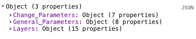
Run CODED by clicking Run. This will set up the run, and issue the call to the ChangeDetection.coded function (Fig. A3.4.6).
Fig. A3.4.6 The result of running the CODED change detection algorithm is an object with the general and change parameters used for the run and a layers object that has all the image outputs |
Code Checkpoint A34d. The book’s repository contains a script that shows what your code should look like at this point.
Next, you will relabel some of the results so that they are easier to understand and work with. You will rename the degradation layers to something more human readable, like ‘degradation_1’, ‘degradation_2’, etc. Rename the deforestation layers to something more human readable, like ‘deforestation_1’, ‘deforestation_2’, etc.
Set a variable for the mask layer. This is the same mask that was passed into CODED, so retrieving it in this method is not strictly necessary.
Set a variable for the change output that is the concatenation of the degradation and deforestation outputs. This is mostly for organizational purposes. Since change is more rare, self masking removes all the non-change pixels, and casting to Int32 helps keep all the bands in the same type, which you would need for exporting to a geoTIFF.
Set a variable mag to the minimum magnitude. There are multiple magnitude bands that correspond to the number of temporal segments that are retrieved when running CODED. These bands are reduced by the minimum since we want to find areas where the greatest negative change has occurred.
// Format the results for exporting. |
Finally, we can combine all of this information into a stratified—or classified—output layer of forest, non-forest, degradation, and deforestation. We can define a function to take in each of the outputs and apply some logic to decide these categories. A new threshold we need to apply is the magnitude, magThreshold. This threshold will define the minimum amount of change we want to qualify as a degradation or deforestation event. This is a post-processing step in which we will stratify the results into categories of stable forest, stable non-forest, degradation, and deforestation.
Next, you will create a new function named makeStrata that takes an image and a threshold as the arguments. The base of the stratified image will be the mask which is remapped from [0,1] to [2,1]. This keeps the forest class at a value of 1 and updates the non-forest class to a value of 2.
Then, you will create a binary mask of the minimum threshold using the magnitude threshold parameter. Then, create a binary degradation image using all the degradation bands and then multiply it by the magnitude mask. Similarly, you’ll create a binary deforestation image using all the deforestation bands and then multiply it by the magnitude mask. Update the strata image using the where functions to first assign degradation to 3 and next to assign deforestation to 4. The where functions are applied sequentially. Deforestation needs to be updated last because in this case, areas of degradation could overlap with areas that are also deforestation.
var makeStrata=function(img, magThreshold){ |
Concatenate the mask, change, and mag bands into a single image. Define a magnitude threshold of -0.6. Apply the makeStrata function using the full output image and the magnitude threshold. Then, add code to export the strata to your assets.
var fullOutput=ee.Image.cat([mask, change, mag]); |
Click Run. The CODED algorithm is computationally heavy, so the results need to be exported before they can be viewed on the map in the Code Editor. Once the export has finished, you can add the layer to the map. We have created the asset for you and stored it in the book repository; you can access it with the code below:
var exportedStrata=ee.Image('projects/gee-book/assets/A3-4/strata'); |
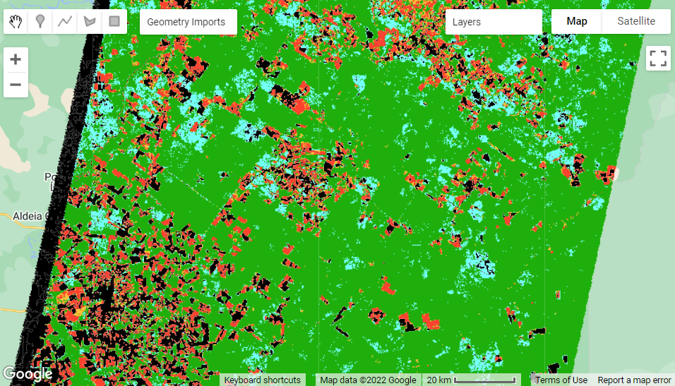
The resulting map should look something like the example in Fig. A3.4.9. With these stratified results, you can see the relative amounts and geographic distribution of forest that have been degraded or deforested in your time period of interest. What patterns do you observe? Does forest degradation or deforestation seem more prevalent?
Fig. A3.4.9 Example of classified CODED results for 1990 to 2020. Non-forested areas are black, stable forest areas are green, deforestation is red, and degradation is yellow. |
Code Checkpoint A34e. The book’s repository contains a script that shows what your code should look like at this point.
Synthesis
Assignment 1. Study how adjusting each parameter affects your results.
- When you decrease the chi-squared probability, do you see more or less deforestation, and more or less degradation?
- When you decrease the magnitude threshold, do you see more or less deforestation, and more or less degradation?
- When you decrease the number of observations, do you see more or less deforestation, and more or less degradation?
Assignment 2. Try adjusting the CODED parameters to see how they affect the detection of degradation and deforestation in a study area where you highly suspect from the imagery that these events have occured. Observe in the map whether you are overestimating or underestimating the disturbed forest area with each parameter combination.
Conclusion
In this chapter you learned about the spectral unmixing algorithm (SMA) and the Normalized Difference Fraction Index (NDFI) in order to map forest degradation and deforestation. We presented two examples of change detection applications: two-image differencing, and an NDFI time-series approach using the CODED algorithm. NDFI is sensitive to subtle changes in forest composition, making it ideal for detection of forest degradation. CODED’s use of a regression model fitting of NDFI over a training period informs us more about what the NDFI magnitudes and variability of a forest should be in a healthy state, so changes from the norm can be more confidently labeled as forest disturbance events. However, your chosen CODED parameters have an important impact on your resulting map of forest loss and forest degradation.
Feedback
To review this chapter and make suggestions or note any problems, please go now to bit.ly/EEFA-review. You can find summary statistics from past reviews at bit.ly/EEFA-reviews-stats.
References
Cloud-Based Remote Sensing with Google Earth Engine. (n.d.). CLOUD-BASED REMOTE SENSING WITH GOOGLE EARTH ENGINE. https://www.eefabook.org/
Cloud-Based Remote Sensing with Google Earth Engine. (2024). In Springer eBooks. https://doi.org/10.1007/978-3-031-26588-4
Adams JB, Sabol DE, Kapos V, et al (1995) Classification of multispectral images based on fractions of endmembers: Application to land-cover change in the Brazilian Amazon. Remote Sens Environ 52:137–154. https://doi.org/10.1016/0034-4257(94)00098-8
Aryal RR, Wespestad C, Kennedy RE, et al (2021) Lessons learned while implementing a time-series approach to forest canopy disturbance detection in Nepal. Remote Sens 13:2666. https://doi.org/10.3390/rs13142666
Asner GP, Keller M, Pereira R, Zweede JC (2002) Remote sensing of selective logging in Amazonia: Assessing limitations based on detailed field observations, Landsat ETM+, and textural analysis. Remote Sens Environ 80:483–496. https://doi.org/10.1016/S0034-4257(01)00326-1
Asner GP, Keller M, Pereira R, et al (2004) Canopy damage and recovery after selective logging in Amazonia: Field and satellite studies. Ecol Appl 14:280–298. https://doi.org/10.1890/01-6019
Bullock E (2018) Background and Motivation — CODED 0.2 Documentation. https://coded.readthedocs.io/en/latest/background.html. Accessed 28 May 2021
Bullock EL, Woodcock CE, Souza C, Olofsson P (2020) Satellite-based estimates reveal widespread forest degradation in the Amazon. Glob Chang Biol 26:2956–2969. https://doi.org/10.1111/gcb.15029
Bullock E, Nolte C, Reboredo Segovia A (2018) Project impact assessment on deforestation and forest degradation: Forest Disturbance Dataset. 1–44
Cochrane MA (1998) Linear mixture model classification of burned forests in the Eastern Amazon. Int J Remote Sens 19:3433–3440. https://doi.org/10.1080/014311698214109
Hansen MC, Potapov P V, Moore R, et al (2013) High-resolution global maps of 21st-century forest cover change. Science 342:850–853. https://doi.org/science.1244693
Hirschmugl M, Steinegger M, Gallaun H, Schardt M (2013) Mapping forest degradation due to selective logging by means of time series analysis: Case studies in Central Africa. Remote Sens 6:756–775. https://doi.org/10.3390/rs6010756
Kusbach A, Friedl M, Zouhar V, et al (2017) Assessing forest classification in a landscape-level framework: An example from Central European forests. Forests 8:461. https://doi.org/10.3390/f8120461
Matricardi EAT, Skole DL, Cochrane MA, et al (2007) Multi-temporal assessment of selective logging in the Brazilian Amazon using Landsat data. Int J Remote Sens 28:63–82. https://doi.org/10.1080/01431160600763014
Schultz M, Clevers JGPW, Carter S, et al (2016) Performance of vegetation indices from Landsat time series in deforestation monitoring. Int J Appl Earth Obs Geoinf 52:318–327. https://doi.org/10.1016/j.jag.2016.06.020
Small C (2004) The Landsat ETM+ spectral mixing space. Remote Sens Environ 93:1–17. https://doi.org/10.1016/j.rse.2004.06.007
Souza Jr CM, Barreto P (2000) An alternative approach for detecting and monitoring selectively logged forests in the Amazon. Int J Remote Sens 21:173–179. https://doi.org/10.1080/014311600211064
Souza Jr CM, Firestone L, Silva LM, Roberts D (2003) Mapping forest degradation in the Eastern Amazon from SPOT 4 through spectral mixture models. Remote Sens Environ 87:494–506. https://doi.org/10.1016/j.rse.2002.08.002
Souza Jr CM, Roberts DA, Cochrane MA (2005) Combining spectral and spatial information to map canopy damage from selective logging and forest fires. Remote Sens Environ 98:329–343. https://doi.org/10.1016/j.rse.2005.07.013
Woodcock CE, Loveland TR, Herold M, Bauer ME (2020) Transitioning from change detection to monitoring with remote sensing: A paradigm shift. Remote Sens Environ 238:111558. https://doi.org/10.1016/j.rse.2019.111558
Zhu Z, Woodcock CE (2014) Continuous change detection and classification of land cover using all available Landsat data. Remote Sens Environ 144:152–171. https://doi.org/10.1016/j.rse.2014.01.011