Cloud-Based Remote Sensing with Google Earth Engine

Fundamentals and Applications

Part A2: Aquatic and Hydrological Applications

Earth Engine’s global scope and long time series allow analysts to understand the water cycle in new and unique ways. These include surface water in the form of floods and river characteristics, long-term issues of water balance, and the detection of subsurface ground water.

Chapter A2.3: Surface Water Mapping

Authors

K. Markert, G. Donchyts, A. Haag

Overview

In this chapter, you will learn the step-by-step implementation of an efficient and robust approach for mapping surface water. You will also learn how the extracted surface water information can be used in conjunction with historical surface water information to extract flooded areas. This chapter will focus mostly on the use of Sentinel-1 Synthetic Aperture Radar (SAR) data, but the approaches apply to both SAR and optical remotely sensed data.

Learning Outcomes

• Applying Otsu thresholding techniques for surface water mapping.
• Understanding the considerations of global versus adaptive histogram sampling.
• Implementing an adaptive histogram sampling approach.
• Extracting flooded areas from a surface water map.

Helps if you know how to:

• ​​Import images and image collections, filter, and visualize (Part F1).
• ​​Create a graph using ui.Chart (Chap. F1.3).
• Write a function and map it over an ImageCollection (Chap. F4.0).
• Understand basics of working with Synthetic Aperture Radar images (Chap. A1.8).

Github Code link for all tutorials

This code base is collection of codes that are freely available from different authors for google earth engine.

Github Source

Introduction to Theory

Flooding impacts more people than any other environmental hazard, and flood exposure is expected to increase in the future (Tellman et al. 2021). Remote sensing data plays a pivotal role in mapping historical flood zones and producing spatial maps of flood events that can be used to guide response efforts (Oddo and Bolten 2019). Oftentimes, flood maps need to be created and delivered to disaster managers within hours of image acquisition. Thus, computationally efficient approaches are required to reduce latency. Furthermore, these approaches need to produce accurate results without increasing processing time.

Image thresholding is an efficient method for mapping surface water (Schumann et al. 2009). Among the numerous methods available for image thresholding, a popular one is “Otsu’s method” (Otsu 1979). Otsu’s method is a histogram-based thresholding approach where the inter-class variance between two classes, a foreground class and a background class, is maximized. As this approach assumes that only two classes are present within an image, which is rarely the case, methods have been developed (Donchyts et al. 2016, Cao et al. 2019) to constrain histogram sampling to areas that are more likely to represent a bimodal histogram of water/no water. Otsu’s method applied on such a constrained histogram provides a more accurate estimation of a water threshold without sacrificing the computational efficiency of the method.

This chapter explores surface water mapping using Otsu’s method, and walks through an adaptive thresholding technique initially developed by Donchyts et al. 2016 and applied on optical imagery, then adapted by Markert et al. 2020 for detecting surface water in SAR imagery. Furthermore, the resulting surface water map will be compared with the Joint Research Centre’s (JRC) Global Surface Water dataset (Pekel et al. 2016) to extract the flooded areas. This chapter will focus on the use of Sentinel-1 (S1) SAR data, but the concepts apply to other satellite imagery where we can distinguish water.

Practicum

Section 1. Otsu Thresholding

Otsu’s method is widely used for determining the optimal threshold of an image with two classes. In this section, we will explore the use of Otsu’s method for segmenting water using an image-wide histogram (also known as a global histogram).

We will start by accessing Sentinel-1 data. We will focus our analysis on Southeast Asia, which experiences yearly flooding and so provides plenty of good test cases. To do this, we will assign the Sentinel-1 collection to a variable and filter by space, time, and metadata properties to get our image for processing.

Now we can add our image to the map.

The map should now have a Sentinel-1 image in Cambodia that looks like Fig. A2.3.1.

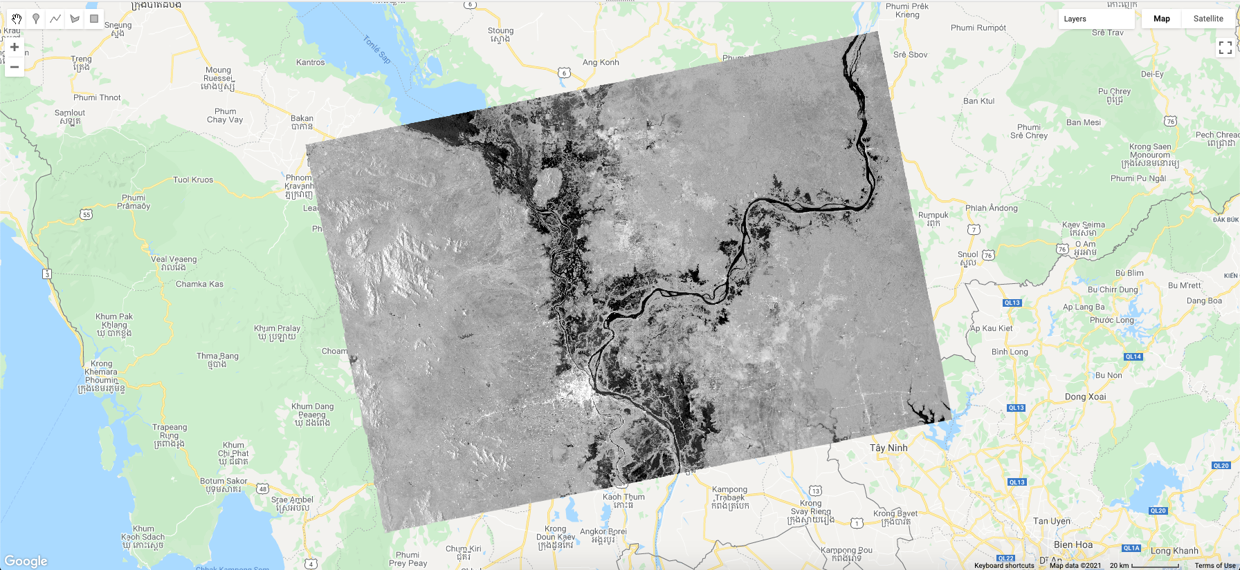
Now that we have our image, we can begin our processing to extract surface water information using Otsu’s threshold. Otsu’s thresholding algorithm uses histograms, so we will need to create one for the pixels of the image.  Otsu’s method works on a single band of values, so we will use the VV band from Sentinel-1, as seen in Fig. A2.3.1. Earth Engine allows us to easily calculate a histogram using the reducer ee.Reducer.histogram applied across the image using the reduceRegion operation:

After running that code, you should see the chart in Fig. A2.3.2 printed in the Console. This is the histogram of values across the image.

In the histogram, the data points are heavily concentrated around −9 dB. We can see a small peak of low backscatter values around −22 dB; these are the likely open-water values. The SAR signal bounces off large, smooth surfaces like water, so likely open-water values are low, and non-water values are high.

How should we split the histogram into two parts to create a high-quality partition of the image into two classes? That is the job of Otsu’s thresholding algorithm. Earth Engine does not have a built-in function for Otsu’s method, so we will create a function that implements the algorithm’s logic. This function takes in a histogram as input, applies the algorithm, and returns a single value where Otsu’s method suggests breaking the histogram into two parts. (More information about Otsu’s method can be found in the “For Further Reading” section of this book.)

When the threshold is calculated, it can be applied to the imagery and we can inspect where it falls within our histogram. The following code creates a new array of values and checks where the threshold is so that we can see how the algorithm performed.

Once you have run the above code, you should see another histogram chart that looks like Fig. A2.3.3. Note the addition of the text and light vertical line indicating the location of the threshold value.

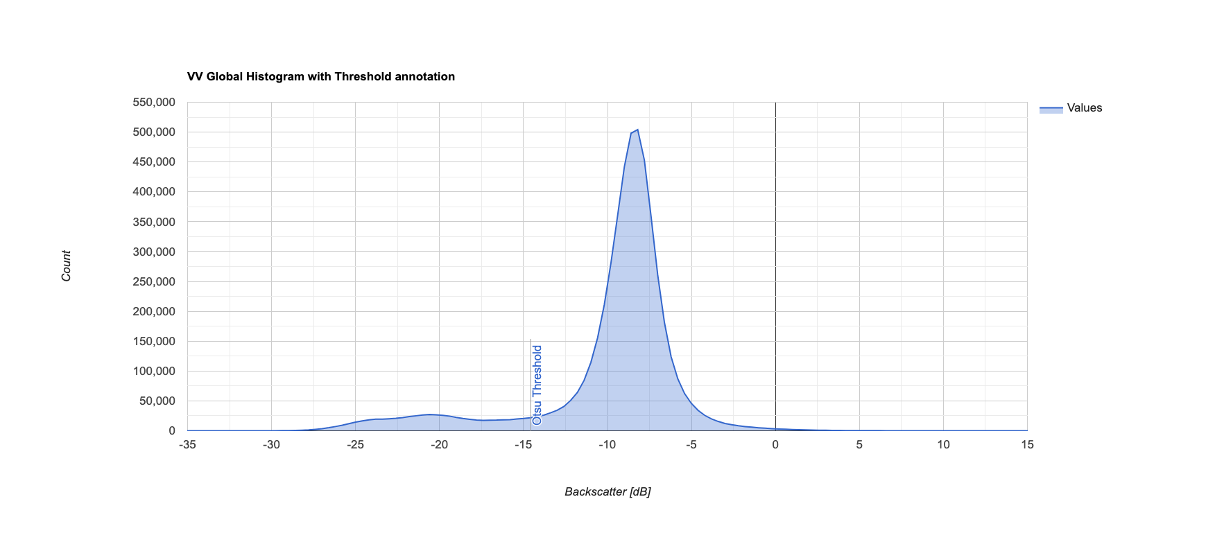
We can see that the threshold is around −15 dB, which is about halfway between the two peaks. We can now apply that threshold on the imagery and inspect how the extracted water looks compared to the original image. Using the code below, we apply the threshold and add the water image to the map.

The results look promising. The blue areas overlap with the low backscatter (specular reflectance) that is representative of open water in C-band SAR imagery. However, upon closer inspection we can see that the extracted water overestimates in some areas.

We see an overestimation as large local errors may be introduced when calculating a constant threshold for distinguishing water from land when using an image-wide histogram. It is due to this issue that algorithms have been developed to constrain the histogram sampling and estimate a more locally contextual threshold.

Code Checkpoint A23a. The book’s repository contains a script that shows what your code should look like at this point.

Question 1. Do some reading on Otsu’s method (the Wikipedia page has a good description). How does Otsu’s threshold work? What underlying assumptions does Otsu’s threshold make?

Question 2. Based on the results and your understanding of Otsu’s thresholding, why do you think the calculated histogram overestimated water areas?

Section 2. Adaptive Thresholding

Surface water usually constitutes only a small fraction of the overall land cover within an Earth observation image. This makes it harder to apply threshold-based methods to extract water. The challenge is to establish a varying threshold that can be derived automatically. In images that show flooding, like the one from the previous section, this limitation is not so significant. Nevertheless, this section walks through an adaptive thresholding technique designed to overcome the challenges of using a global threshold.

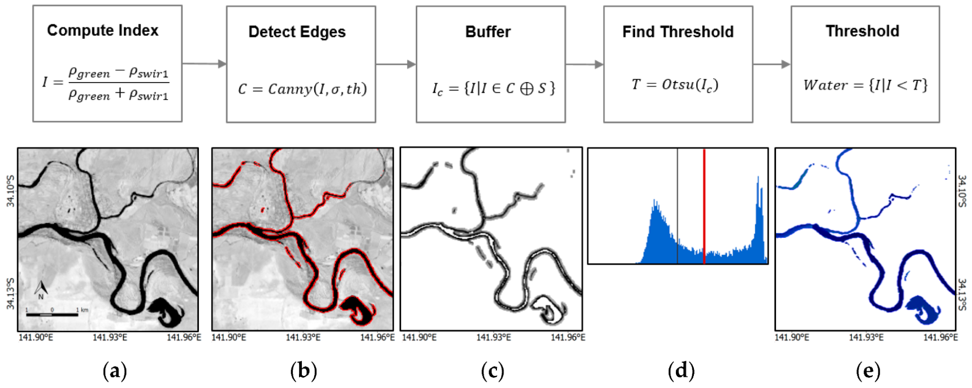
The method we will discuss was developed by Donchyts et al. (2016) and applied to the Modified Normalized Difference Water Index (MNDWI) from Landsat 8 imagery. The algorithm finds edges within the image, buffers the areas around the identified edges, and uses the buffered area to sample a histogram for Otsu thresholding. This approach assumes that the edges detected are from water. The result is a bimodal histogram from the area around water edges that can be used to calculate a refined threshold. The overall workflow of the algorithm is shown in Fig. A2.3.6.

This approach was refined by Markert et al. (2020), where the main change is that instead of calculating the edges on the raw values (from an index or otherwise), an initial segmentation threshold is provided to create a binary image as input for the edge detection. This overcomes issues with SAR speckle and other artifacts, as well as with any edges being defined from other classes that are present in imagery (e.g., urban areas or forests). The defined edges are then filtered by length to omit small edges that can occur and can skew the histogram sampling. This requires that a few parameters be tuned, namely the initial threshold, edge length, and buffer size. Here, we define a few of those parameters.

With these parameters defined, we can begin the process of constraining the histogram sampling.

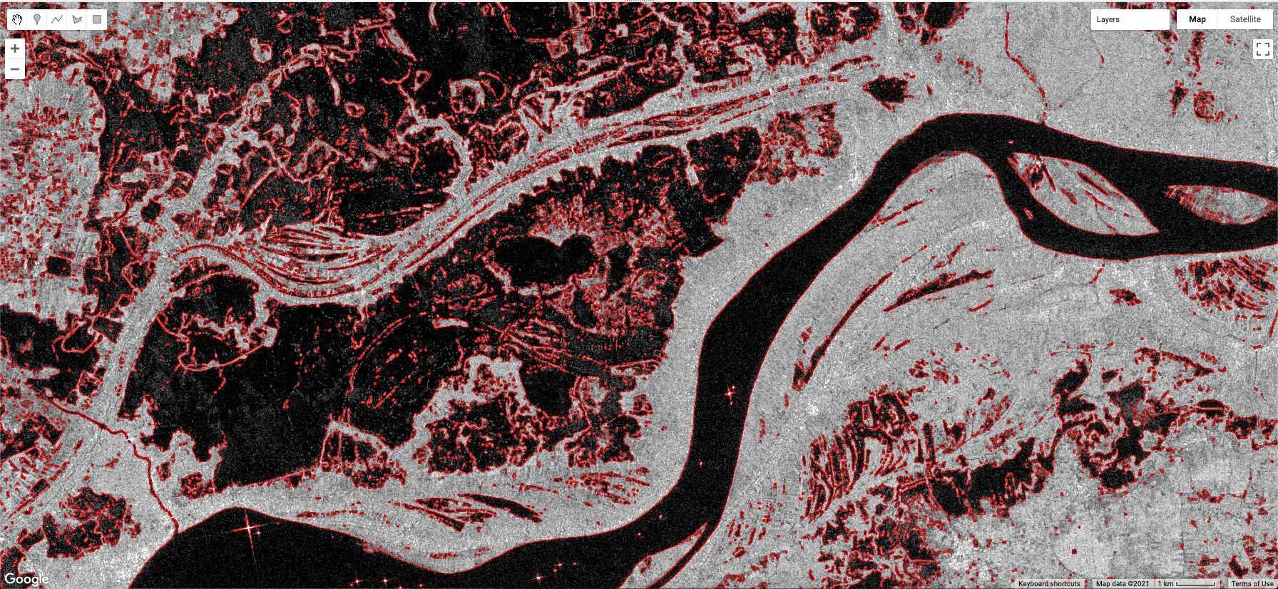
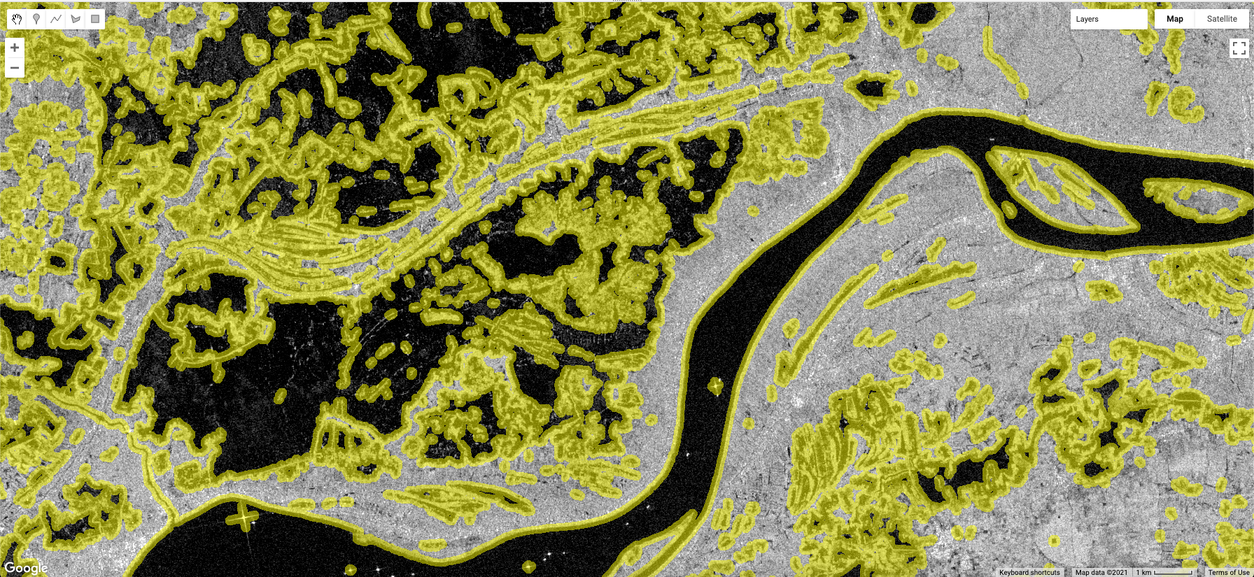
Now that we have the edge information and the data to sample processed, we can visually inspect what the algorithm is doing. Here, we will display the calculated edges as well as the buffered edges to highlight which data is being sampled.

You should now have the data added to the map, which should look like the images in Fig. 2.3.7 when zoomed in.

At this point, we have our regions that we want to sample that are more representative of a bimodal histogram, and we have masked out areas that we don’t want to sample. Now we can calculate the histogram as before and make a plot.

We can see from the histogram that we have two distinct peaks. This meets the assumption of Otsu thresholding that only two classes are present within an image, which allows the algorithm to more accurately calculate the threshold for water. The last thing left to do is to apply the calculated adaptive threshold on the imagery and add it to the map.

It can be seen from the resulting images that the adaptive thresholding technique produces a reasonable surface water map. Furthermore, the resulting threshold value was −15.799, as compared to −14.598 from the global thresholding. A lower threshold in this case means less surface water area extracted. However, less surface water area does not necessarily mean more accuracy. There needs to be a balance between producer’s and user’s accuracy.

Now that we have a surface water map and we are moderately confident that it represents the actual surface water for that day, we can begin to identify flooded areas by differencing our map with historical information.

Code Checkpoint A23b. The book’s repository contains a script that shows what your code should look like at this point.

Question 3. Why do we apply an initial threshold to the SAR imagery prior to detecting edges? What happens to the detected edges if we do not apply an initial threshold? Explain why you are or are not getting a difference in detected edges. Recall that we defined some parameters for the Canny edge detection. Show a comparison.

Question 4. Compare the threshold calculated with the adaptive technique to the global threshold. In your own words, explain why the two thresholds are different.

Question 5. Change the parameters used for the adaptive thresholding to see how the results change. Which parameters is the algorithm most sensitive to?

Section 3. Extracting Flood Areas

Up to this point, we have been mapping surface water, which includes permanent and seasonal water that was observed by the sensor. What we need to do now is to identify areas from our image that are considered permanent water. There are typically two approaches to mapping flooded areas with a thematic surface water map: (1) comparing pre- and post-event images to estimate changes; or (2) comparing extracted surface water with historically observed permanent water.

To achieve the goal of flood mapping, we will use the historical JRC Global Surface Water dataset to define permanent water and then find the difference to extract flooded areas. We already have our post-event surface water map. Now we need to access and use the JRC data.

Because this data is a yearly classification of permanent and seasonal water, we need to reclassify the imagery to just permanent water.

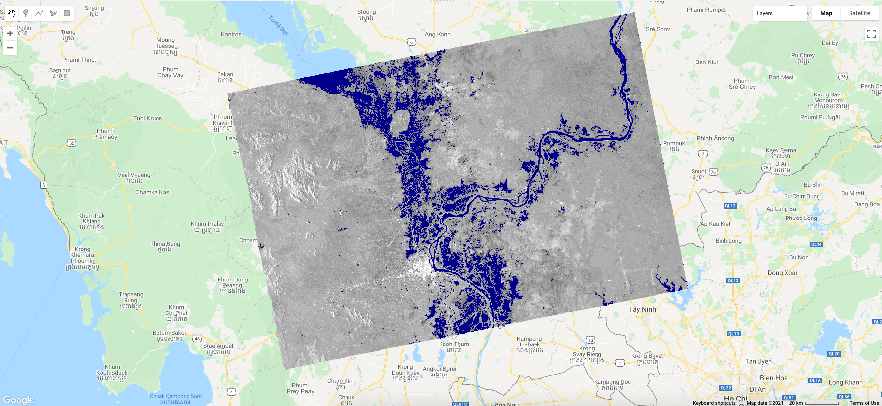
The final thing we need to do is apply a simple differencing between the surface water map from Sentinel-1 and the JRC permanent water.

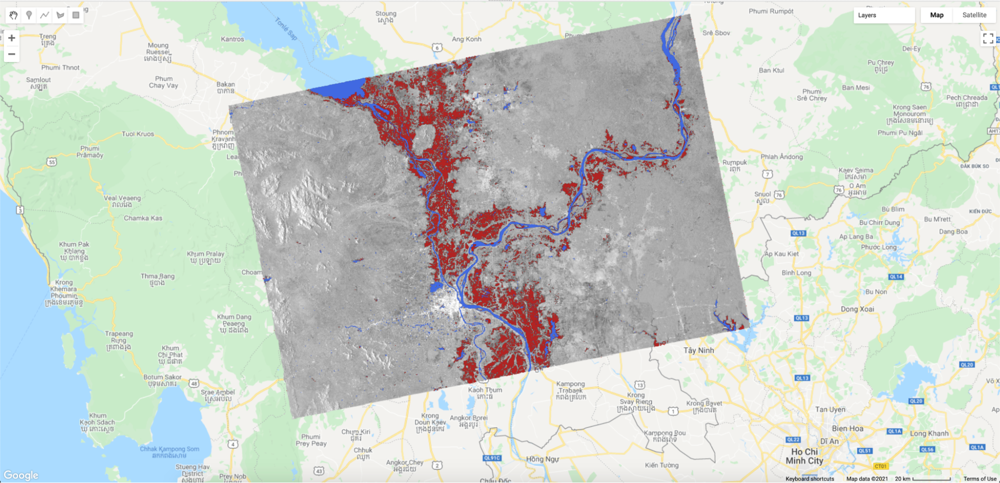
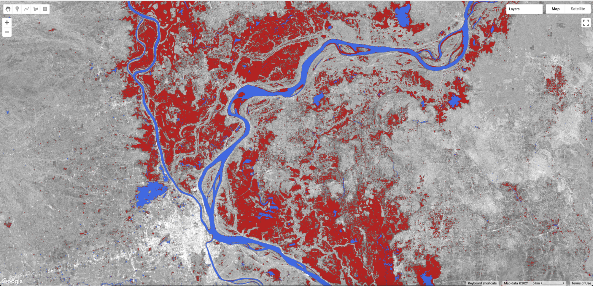
There are nuances associated with comparing optically derived water information (like from JRC) with SAR water maps. For example, any surface that is large enough and smooth can “look” like water in SAR imagery because of specular reflectance and can be wrongly classified as a flooded area. Examples of this are airports, exposed channel beds, and highways. It should also be noted that there is a component of seasonal flooding—flooding that occurs every year and is expected. Currently, our flood map contains areas of seasonal flooding as well. Therefore, to accurately map the “abnormal” area of a flood, we’d also have to account for seasonal patterns. Lastly, rivers are in constant flux, changing patterns, and even change due to flooding events, so comparing historical observations with flooding events may yield some areas that have changed. Therefore, comparing pre- and post-event imagery from the same sensor is best. However, it is challenging to define events in seasonal flooding (such as this case), making a pre- and post-event comparison a little more complicated.

Code Checkpoint A23c. The book’s repository contains a script that shows what your code should look like at this point.

Synthesis

In this chapter, we covered a common image segmentation method, Otsu’s thresholding, and applied it to map surface water using Sentinel-1 SAR imagery. Furthermore, we illustrated an image processing technique to constrain the histogram sampling for input into the Otsu thresholding method. Lastly, we created a flood map from the segmented surface water map using historical permanent surface water data. You should now have a good grasp on the Otsu thresholding technique for surface water mapping, understand the considerations of global versus localized histogram sampling, be able to implement an adaptive histogram sampling approach, and take a surface water map and convert it to a flood map.

Assignment 1. Identify a flooding event of interest (a good source is https://floodlist.com) and walk through the process of creating a flood map for the event you chose. Do you notice anything different with the resulting flood map? Make note of the identified threshold value. Does the threshold value represent water versus no-water areas? Keep in mind the physical properties of SAR—some areas naturally have low backscatter like water does.

Assignment 2.  In your own words, describe the difference between a surface water map and a flood map. Conceptually, what do you need to take into consideration when extracting flood areas?

Assignment 3. Find a pre-event Sentinel-1 image for the case we have gone through, extract surface water from the pre-event image, and compare it to the post- event image. Do you find differences in the flood areas derived from pre/post comparison versus historical comparison?

Assignment 4. Refactor the code to make the adaptive thresholding algorithm and flood mapping into a callable function that can be mapped over an image collection.

Conclusion

It should be noted that Sentinel-1 SAR imagery ideally should undergo preprocessing to remove the effects of terrain and speckle in imagery, as in Mullissa et al. (2021), before applying surface water mapping algorithms. However, SAR preprocessing is outside the scope of this chapter.

There are many more sophisticated algorithms for mapping surface water from satellite imagery (such as Mayer et al. 2021). The application illustrated in this chapter is meant to highlight a practical workflow for mapping surface water and floods that can be implemented in Earth Engine.

Feedback

To review this chapter and make suggestions or note any problems, please go now to bit.ly/EEFA-review. You can find summary statistics from past reviews at bit.ly/EEFA-reviews-stats.

References

Cloud-Based Remote Sensing with Google Earth Engine. (n.d.). CLOUD-BASED REMOTE SENSING WITH GOOGLE EARTH ENGINE. https://www.eefabook.org/

Cloud-Based Remote Sensing with Google Earth Engine. (2024). In Springer eBooks. https://doi.org/10.1007/978-3-031-26588-4

Cao H, Zhang H, Wang C, Zhang B (2019) Operational flood detection using Sentinel-1 SAR data over large areas. Water (Switzerland) 11:786. https://doi.org/10.3390/w11040786

Donchyts G, Schellekens J, Winsemius H, et al (2016) A 30 m resolution surface water mask including estimation of positional and thematic differences using Landsat 8, SRTM and OpenStreetMap: A case study in the Murray-Darling basin, Australia. Remote Sens 8:386. https://doi.org/10.3390/rs8050386

Markert KN, Markert AM, Mayer T, et al (2020) Comparing Sentinel-1 surface water mapping algorithms and radiometric terrain correction processing in Southeast Asia utilizing Google Earth Engine. Remote Sens 12:2469. https://doi.org/10.3390/RS12152469

Mayer T, Poortinga A, Bhandari B, et al (2021) Deep learning approach for Sentinel-1 surface water mapping leveraging Google Earth Engine. ISPRS Open J Photogramm Remote Sens 2:100005. https://doi.org/10.1016/j.ophoto.2021.100005

Mullissa A, Vollrath A, Odongo-Braun C, et al (2021) Sentinel-1 SAR backscatter analysis ready data preparation in Google Earth Engine. Remote Sens 13:1954. https://doi.org/10.3390/rs13101954

Oddo PC, Bolten JD (2019) The value of near real-time Earth observations for improved flood disaster response. Front Environ Sci 7:127. https://doi.org/10.3389/fenvs.2019.00127

Otsu N (1979) A threshold selection method from gray-level histograms. IEEE Trans Syst Man Cybern SMC-9:62–66. https://doi.org/10.1109/tsmc.1979.4310076

Pekel JF, Cottam A, Gorelick N, Belward AS (2016) High-resolution mapping of global surface water and its long-term changes. Nature 540:418–422. https://doi.org/10.1038/nature20584

Schumann G, Di Baldassarre G, Bates PD (2009) The utility of spaceborne radar to render flood inundation maps based on multialgorithm ensembles. IEEE Trans Geosci Remote Sens 47:2801–2807. https://doi.org/10.1109/TGRS.2009.2017937

Tellman B, Sullivan JA, Kuhn C, et al (2021) Satellite imaging reveals increased proportion of population exposed to floods. Nature 596:80–86. https://doi.org/10.1038/s41586-021-03695-w