Cloud-Based Remote Sensing with Google Earth Engine

Fundamentals and Applications

Part F3: Advanced Image Processing

Once you understand the basics of processing images in Earth Engine, this Part will present some of the more advanced processing tools available for treating individual images. These include creating regressions among image bands, transforming images with pixel-based and neighborhood-based techniques, and grouping individual pixels into objects that can then be classified.

Chapter F3.0: Interpreting an Image: Regression

Authors

Karen Dyson, Andréa Puzzi Nicolau, David Saah, Nicholas Clinton

Overview

This chapter introduces the use of regression to interpret imagery. Regression is one of the fundamental tools you can use to move from viewing imagery to analyzing it. In the present context, regression means predicting a numeric variable for a pixel instead of a categorical variable, such as a class label.

Learning Outcomes

• Learning about Earth Engine reducers.
• Understanding the difference between regression and classification.
• Using reducers to implement regression between image bands.
• Evaluating regression model performance visually and numerically.

Assumes you know how to:

• Import images and image collections, filter, and visualize (Part F1).
• Perform basic image analysis: select bands, compute indices, create masks (Part F2).
• Understand the characteristics of Landsat data and MODIS data (Chap. F1.2, Chap. F1.3).
• Use normalizedDifference to calculate vegetation indices (Chap. F2.0).
• Interpret variability of the NDVI, the Normalized Difference Vegetation Index (Chap. F2.0).
• Have an understanding of regression.

Github Code link for all tutorials

This code base is collection of codes that are freely available from different authors for google earth engine.

Github Source

Introduction to Theory

If you have already used regression in other contexts, this approach will be familiar to you. Regression in remote sensing uses the same basic concepts as regression in other contexts. We determine the strength and characteristics of the relationship between the dependent variable and one or more independent variables to better understand or forecast the dependent variable. In a remote sensing context, these dependent variables might be the likelihood of a natural disaster or a species occurrence, while independent variables might be bands, indices, or other raster datasets like tree height or soil type.

Importantly, we use regression for numeric dependent variables. Classification, which is covered in Chap. F2.1, is used for categorical dependent variables, such as land cover or land use.

Regression in remote sensing is a very powerful tool that can be used to answer many important questions across large areas. For example, in China, researchers used a random forest regression algorithm to estimate above-ground wheat biomass based on vegetation indices (Zhou et al. 2016). In the United States, researchers used regression to estimate bird species richness based on lidar measurements of forest canopy (Goetz et al. 2007). In Kenya, researchers estimated tree species diversity using vegetation indices including the tasseled cap transformation and simple and multivariate regression analysis (Maeda et al. 2014).

Practicum

In general, regression in remote sensing follows a standard set of steps. 

1. Data about known instances of the dependent variable are collected. This might be known landslide areas, known areas of species occurrence, etc.
2. The independent variables are defined and selected.
3. A regression is run to generate an equation that describes the relationship between dependent and independent variables.
4. Optional: Using this equation and the independent variable layers, you create a map of the dependent variable over the entire area.

While this set of steps remains consistent across regressions, there are multiple types of regression functions to choose from, based on the properties of your dependent and independent variables, and how many independent variables you have. The choice of regression type in remote sensing follows the same logic as in other contexts. There are many other excellent online resources and textbooks to help you better understand regression and make your choice of regression method. Here, we will focus on running regression in Google Earth Engine and some of the different options available to you.

Reducers

A key goal of working with remote-sensing data is summarizing over space, time, and band information to find relationships. Earth Engine provides a large set of summary techniques for remote-sensing data, which fall under the collective term reducers.

An example of a reducer of a set of numbers is the median, which finds the middle number in a set, reducing the complexity of the large set to a representative estimate. That reducing operation is implemented in Earth Engine with ee.Reducer.median., or for this particularly common operation, with the shorthand operation median.

Reducers can operate on a pixel-by-pixel basis, or with awareness of a pixel’s surroundings. An example of a reducer of a spatial object is computing the median elevation in a neighborhood, which can be implemented in Earth Engine by embedding the call to ee.Reducer.median inside a reduceRegion function. The reduceRegion call directs Earth Engine to analyze pixels that are grouped across an area, allowing an area like a city block or park boundary to be considered as a unified unit of interest. Reducers can be used to summarize many forms of data in Earth Engine, including image collections, images, lists, and feature collections. They are encountered throughout the rest of this book in a wide variety of settings.

Reducers can be relatively simple, like the median, or more complex. Imagine a 1000-person sample of height and weight of individuals: a linear regression would reduce the 2000 assembled values to just two: the slope and the intercept. Of course the relationship might be weak or strong in a given set; the bigger idea is that many operations of simplifying and summarizing large amounts of data can be conceptualized using this idea and terminology of reducers.

In this chapter we will illustrate reducers through their use in regressions of bands in a single image, and revisit regressions using analogous operations on time series in other parts of the book.

Section 1. Linear Fit

If you have not already done so, be sure to add the book’s code repository to the Code Editor by entering https://code.earthengine.google.com/?accept_repo=projects/gee-edu/book into your browser. The book’s scripts will then be available in the script manager panel.

The simplest regression available in Earth Engine is implemented through the reducer linearFit. This function is a least-squares estimate of a linear function with one independent variable and one dependent variable. This regression equation is written  , where  is the intercept of the line and is the slope, Y is the dependent variable, X is the independent variable, and is the error.

Suppose the goal is to estimate percent tree cover in each Landsat pixel, based on known information about Turin, Italy. Below, we will define a geometry that is a rectangle around Turin, and name it Turin.

We need to access data to use as our dependent variable. For this example, we will use the “MOD44B.006 Terra Vegetation Continuous Fields Yearly Global 250m” dataset. Add the code below to your script.

Note: If the path to that ImageCollection were to change, you would get an error when trying to access it. If this happens, you can search for “vegetation continuous MODIS” to find it. Then, you could import it and change its name to mod44b. This has the same effect as the one line above.

Next, we will access that part of the ImageCollection that represents the global percent tree cover at 250 m resolution from 2020. We’ll access the image from that time period using the filterDate command, convert that single image to an Image type using the first command, clip it to Turin, and select the appropriate band. We then print information about the new image percentTree2020 to the Console.

Now we need to access data to use as our independent variables. For this example, we will use the  “USGS Landsat 8 Collection 2 Tier 1 and Real-Time Data Raw Scenes.” Add the code below to your script.

Note: If the path to that ImageCollection changes, you will get an error when trying to access it. If this happens, you can search for “landsat 8 raw” to find it. Then, import it and change its name  to landsat8_raw.

We also need to filter this collection by date and location. We will filter the collection to a clear (cloud-free) date in 2020, and then filter by location.

Using the centroid function will select images that intersect with the center of our Turin geometry, instead of anywhere in the geometry.

Note that we are using a single image for the purposes of this exercise, but in practice you will almost always need to filter an image collection to the boundaries of your area of interest and then create a composite. In that case, you would use a compositing Earth Engine algorithm to get a cloud-free composite of Landsat imagery. If you’re interested in learning more about working with clouds, please see Chap. F4.3.

Use the bands of the Landsat image to calculate NDVI, which we will use as the independent variable:

Now we begin to assemble our data in Earth Engine into the correct format. First, use the addBands function to create an image with two bands: first, the image ndvi, which will act as the independent variable; and second, the image percentTree2020 created earlier.

Now we can set up and run the regression, using the linear fit reducer over our geometry, and print the results. Since building the regression model requires assembling points from around the image for consideration, it is implemented using reduceRegion rather than reduce (see also Part F5). We need to include the scale variable (here 30 m, which is the resolution of Landsat).

Note the parameter bestEffort in the request to ee.Reducer.linearFit . What does it mean? If you had tried to run this without the bestEffort: true argument, you would most likely get an error: “Image.reduceRegion: Too many pixels in the region.” This means that the number of pixels involved has surpassed Earth Engine's default maxPixels limit of 10 million. The reason is the complexity of the regression we are requesting. If you’ve ever done a regression using, say, 100 points, you may have seen or made a scatter plot with the 100 points on it; now imagine a scatter plot with more than 10 million points to envision the scale of what is being requested. Here, the limitation is not Earth Engine’s computing capacity, but rather it is more like a notification that the code is calling for an especially large computation, and that a novice user may not be entirely intending to do something of that complexity. The error text points to several ways to resolve this issue. First, we could increase maxPixels. Second, we could aggregate at a lower resolution (e.g., increase scale from 30 m to 50 m). Third, we could set the bestEffort parameter to true as we do here, which directs the reducer to use the highest resolution for scale without going above maxPixels. Fourth, we could reduce the area for the region (that is, make the study area around Turin smaller). Finally, we could randomly sample the image stack and use that sample for the regression.

Finally, let’s apply the regression to the whole NDVI area, which is larger than our Turin boundary polygon. The calculation is done with an expression, which will be explained further in Chap. F3.1.

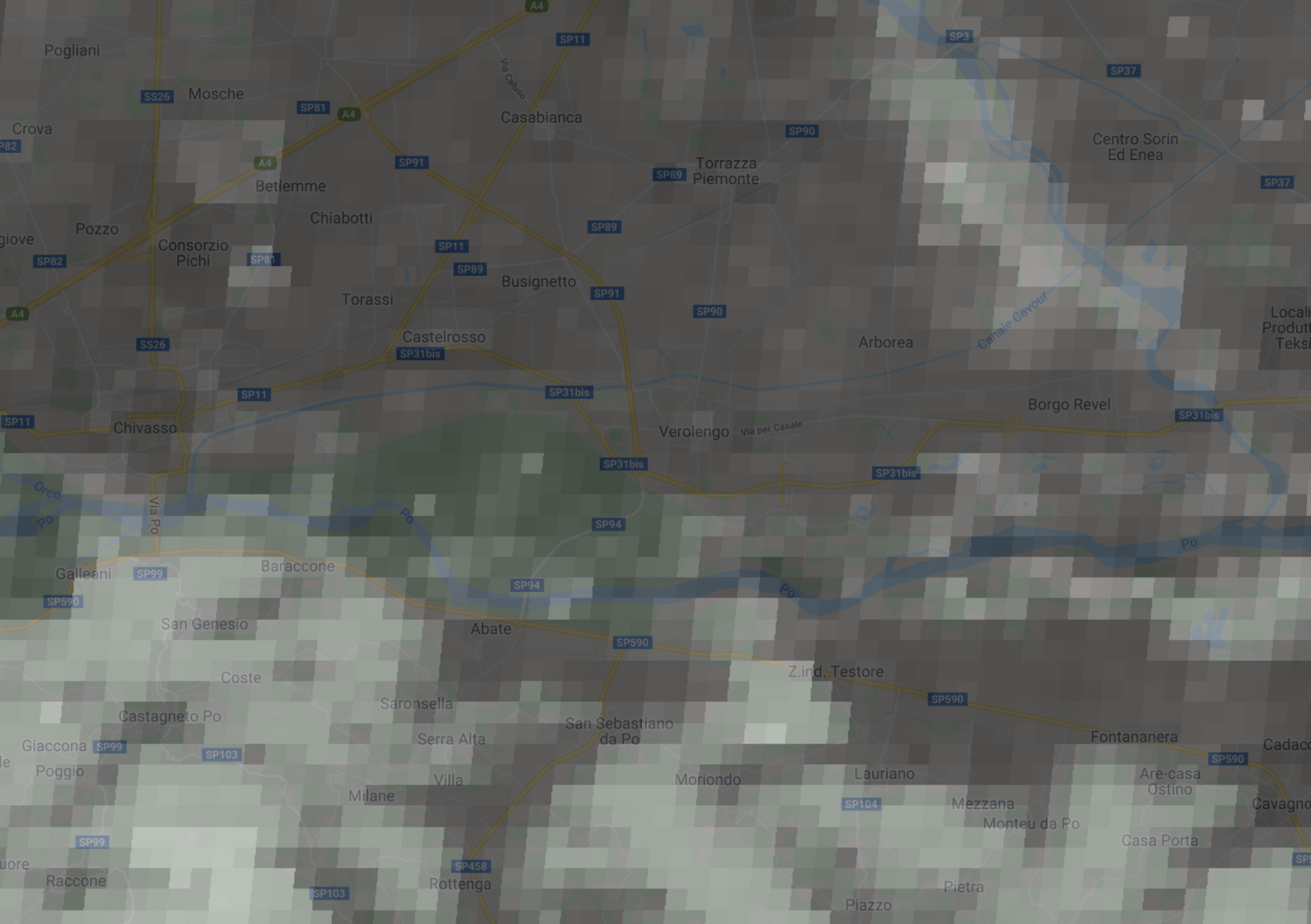
Your estimates based on NDVI are a higher resolution than the MODIS data because Landsat is 30 m resolution. Notice where your estimates agree with the MODIS data and where they disagree, if anywhere. In particular, look at areas of agriculture. Since NDVI doesn’t distinguish between trees and other vegetation, our model will estimate that agricultural areas have higher tree cover percentages than the MODIS data (you can use the Inspector tool to verify this).

Code Checkpoint F30a. The book’s repository contains a script that shows what your code should look like at this point.

Section 2. Linear Regression

The linear regression reducer allows us to increase the number of dependent and independent variables. Let’s revisit our model of percent cover and try to improve on our linear fit attempt by using the linear regression reducer with more independent variables.

We will use our percentTree dependent variable.

For our independent variable, let’s revisit our Landsat 8 image collection. Instead of using only NDVI, let’s use multiple bands. Define these bands to select:

Now let’s assemble the data for the regression. For the constant term needed by the linear regression, we use the ee.Image function to create an image with the value (1) at every pixel. We then stack this constant with the Landsat prediction bands and the dependent variable (percent tree cover).

Inspect your training image to make sure it has multiple layers: a constant term, your independent variables (the Landsat bands), and your dependent variable.

Now we’ll implement the ee.Reducer.linearRegression reducer function to run our linear regression. The reducer needs to know how many X, or independent variables, and the number of Y, or dependent variables, you have. It expects your independent variables to be listed first. Notice that we have used reduceRegion rather than just reduce. This is because we are reducing over the Turin geometry, meaning that the reducer’s activity is across multiple pixels comprising an area, rather than “downward” through a set of bands or an ImageCollection. As mentioned earlier, you will likely get an error that there are too many pixels included in your regression if you do not use the bestEffort variable.

There is also a robust linear regression reducer (ee.Reducer.robustLinearRegression). This linear regression approach uses regression residuals to de-weight outliers in the data following (O’Leary 1990).

Let’s inspect the results. We’ll focus on the results of linearRegression, but the same applies to inspecting the results of the robustLinearRegression reducer.

The output is an object with two properties. First is a list of coefficients (in the order specified by the inputs list) and second is the root-mean-square residual.

To apply the regression coefficients to make a prediction over the entire area, we will first turn the output coefficients into an image, then perform the requisite math.

This code extracts the coefficients from our linear regression and converts them to a list. When we first extract the coefficients, they are in a matrix (essentially 10 lists of 1 coefficient). We use project to remove one of the dimensions from the matrix so that they are in the correct data format for subsequent steps.

Now we will create the predicted tree cover based on the linear regression. First, we create an image stack starting with the constant (1) and use addBands to add the prediction bands. Next, we multiply each of the coefficients by their respective X (independent variable band) using multiply and then sum all of these using ee.Reducer.sum in order to create the estimate of our dependent variable. Note that we are using the rename function to rename the band (if you don’t rename the band, it will have the default name "sum" from the reducer function).

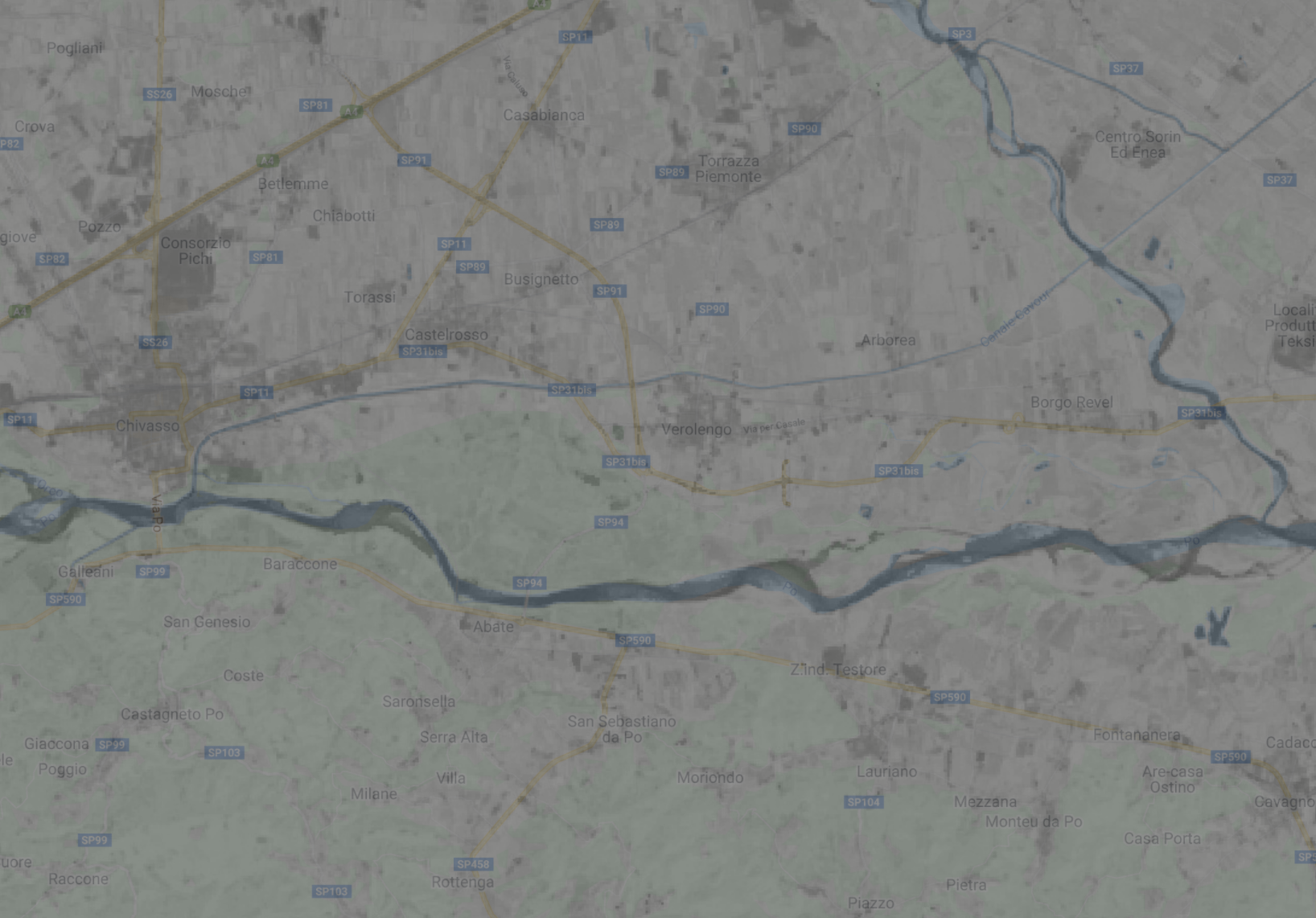
Carefully inspect this result using the satellite imagery provided by Google and the input Landsat data. Does the model predict high forest cover in forested areas? Does it predict low forest cover in unforested areas, such as urban areas and agricultural areas? Note where the model is making mistakes. Are there any patterns? For example, look at the mountainous slopes. One side has a high value and the other side has a low value for predicted forest cover. However, it appears that neither side of the mountain has vegetation above the treeline. This suggests a fault with the model having to do with the aspect of the terrain (the compass direction in which the terrain surface faces) and some of the bands used.

When you encounter model performance issues that you find unsatisfactory, you may consider adding or subtracting independent variables, testing other regression functions, collecting more training data, or all of the above.

Code Checkpoint F30b. The book’s repository contains a script that shows what your code should look like at this point.

Section 3. Nonlinear Regression

Earth Engine also allows the user to perform nonlinear regression. Nonlinear regression allows for nonlinear relationships between the independent and dependent variables. Unlike linear regression, which is implemented via reducers, this nonlinear regression function is implemented by the classifier library. The classifier library also includes supervised and unsupervised classification approaches that were discussed in Chap. F2.1 as well as some of the tools used for accuracy assessment in Chap. F2.2.

For example, a classification and regression tree (CART; see Breiman et al. 2017) is a machine learning algorithm that can learn nonlinear patterns in your data. Let's reuse our dependent variables and independent variables (Landsat prediction bands) from above to train the CART in regression mode.

For CART we need to have our input data as a feature collection. For more on feature collections, see the chapters in Part F5. Here, we first need to create a training data set based on the independent and dependent variables we used for the linear regression section. We will not need the constant term.

Now sample the image stack to create the feature collection training data needed. Note that we could also have used this approach in previous regressions instead of the bestEffort approach we did use.

Now run the regression. The CART regression function must first be trained using the trainingData. For the train function, we need to provide the features to use to train (trainingData), the name of the dependent variable (classProperty), and the name of the independent variables (inputProperties). Remember that you can find these band names if needed by inspecting the trainingData item.

Now we can use this object to make predictions over the input imagery and display the result:

Turn on the satellite imagery from Google and examine the output of the CART regression using this imagery and the Landsat 8 imagery.

Section 4. Assessing Regression Performance Through RMSE

A standard measure of performance for regression models is the root-mean-square error (RMSE), or the correlation between known and predicted values. The RMSE is calculated as follows:

        (F3.0.1)

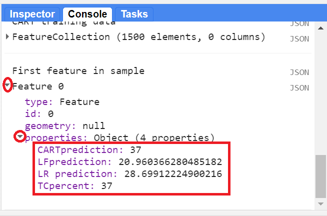
To assess the performance, we will create a sample from the percent tree cover layer and from each regression layer (the predictions from the linear fit, the linear regression, and CART regression). First, using the ee.Image.cat function, we will concatenate all of the layers into one single image where each band of this image contains the percent tree cover and the predicted values from the different regressions. We use the rename function (Chap. F1.1) to rename the bands to meaningful names (tree cover percentage and each model). Then we will extract 500 sample points (the “n” from the equation above) from the single image using the sample function to calculate the RMSE for each regression model. We print the first feature from the sample collection to visualize its properties—values from the percent tree cover and regression models at that point (Fig. F3.0.3), as an example.

In Earth Engine, the RMSE can be calculated by steps. We first define a function to calculate the squared difference between the predicted value and the actual value. We do this for each regression result.

Now, we can apply this function to our sample and use the reduceColumns function to take the mean value of the squared differences and then calculate the square root of the mean value.

Note the following (do not worry too much about fully understanding each item at this stage of your learning; just keep in mind that this code block calculates the RMSE value):

• We start by casting an ee.List since we are calculating three different values—which is also the reason to cast ee.Number at the beginning. Also, it is not possible to map a function to a ee.Number object—another reason why we need the ee.List.
• Since we have three predicted values we used repeat(3) for the reducer parameter of the reduceColumns function—i.e., we want the mean value for each of the selectors (the squared differences).
• The direct output of reduceColumns is a dictionary, so we need to use get('mean') to get these specific key values.
• At this point, we have a “list of lists,” so we use flatten to dissolve it into one list
• Finally, we map the function to calculate the square root of each mean value for the three results.
• The RMSE values are in the order of the selectors; thus, the first value is the linear fit RMSE, followed by the linear regression RMSE, and finally the CART RMSE.

Inspect the RMSE values on the Console. Which regression performed best? The lower the RMSE, the better the result.

Code Checkpoint F30c. The book’s repository contains a script that shows what your code should look like at this point.

Synthesis

Assignment 1. Examine the CART output you just created. How does the nonlinear CART output compare with the linear regression we ran previously? Use the inspect tool to check areas of known forest and non-forest (e.g., agricultural and urban areas). Do the forested areas have a high predicted percent tree cover (will display as white)? Do the non-forested areas have a low predicted percent tree cover (will display as black)? Do the alpine areas have low predicted percent tree cover, or do they have the high/low pattern based on aspect seen in the linear regression?

Assignment 2. Revisit our percent tree cover regression examples. In these, we used a number of bands from Landsat 8, but there are other indices, transforms, and datasets that we could use for our independent variables.

For this assignment, work to improve the performance of this regression. Consider adding or subtracting independent variables, testing other regression functions, using more training data (a larger geometry for Turin), or all of the above. Don’t forget to document each of the steps you take. What model settings and inputs are you using for each model run?

To improve the model, think about what you know about tree canopies and tree canopy cover. What spectral signature do the deciduous trees of this region have? What indices are useful for detecting trees? How do you distinguish trees from other vegetation? If the trees in this region are deciduous, what time frame would be best to use for the Landsat 8 imagery? Consider seasonality—how do these forests look in summer vs. winter?

Practice your visual assessment skills. Ask critical questions about the results of your model iterations. Why do you think one model is better than another?

Conclusion

Regression is a fundamental tool that you can use to analyze remote sensing imagery. Regression specifically allows you to analyze and predict numeric dependent variables, while classification allows for the analysis and prediction of categorical variables (see Chap. F2.1). Regression analysis in Earth Engine is flexible and implemented via reducers (linear regression approaches) and via classifiers (nonlinear regression approaches). Other forms of regression will be discussed in Chap. F4.6 and the chapters that follow. 

Feedback

To review this chapter and make suggestions or note any problems, please go now to bit.ly/EEFA-review. You can find summary statistics from past reviews at bit.ly/EEFA-reviews-stats.

References

Cloud-Based Remote Sensing with Google Earth Engine. (n.d.). CLOUD-BASED REMOTE SENSING WITH GOOGLE EARTH ENGINE. https://www.eefabook.org/

Cloud-Based Remote Sensing with Google Earth Engine. (2024). In Springer eBooks. https://doi.org/10.1007/978-3-031-26588-4

Breiman L, Friedman JH, Olshen RA, Stone CJ (2017) Classification and Regression Trees. Routledge

Goetz S, Steinberg D, Dubayah R, Blair B (2007) Laser remote sensing of canopy habitat heterogeneity as a predictor of bird species richness in an eastern temperate forest, USA. Remote Sens Environ 108:254–263. https://doi.org/10.1016/j.rse.2006.11.016

Maeda EE, Heiskanen J, Thijs KW, Pellikka PKE (2014) Season-dependence of remote sensing indicators of tree species diversity. Remote Sens Lett 5:404–412. https://doi.org/10.1080/2150704X.2014.912767

O’Leary DP (1990) Robust regression computation using iteratively reweighted least squares. SIAM J Matrix Anal Appl 11:466–480. https://doi.org/10.1137/0611032

Zhou X, Zhu X, Dong Z, et al (2016) Estimation of biomass in wheat using random forest regression algorithm and remote sensing data. Crop J 4:212–219. https://doi.org/10.1016/j.cj.2016.01.008