Cloud-Based Remote Sensing with Google Earth Engine
Fundamentals and Applications

Part F4: Interpreting Image Series
One of the paradigm-changing features of Earth Engine is the ability to access decades of imagery without the previous limitation of needing to download all the data to a local disk for processing. Because remote-sensing data files can be enormous, this used to limit many projects to viewing two or three images from different periods. With Earth Engine, users can access tens or hundreds of thousands of images to understand the status of places across decades.
Chapter F4.4: Change Detection
Authors
Karis Tenneson, John Dilger, Crystal Wespestad, Brian Zutta, Andréa P Nicolau, Karen Dyson, Paula Paz
Overview
This chapter introduces change detection mapping. It will teach you how to make a two-date land cover change map using image differencing and threshold-based classification. You will use what you have learned so far in this book to produce a map highlighting changes in the land cover between two time steps. You will first explore differences between the two images extracted from these time steps by creating a difference layer. You will then learn how to directly classify change based on the information in both of your images.
Learning Outcomes
- Creating and exploring how to read a false-color cloud-free Landsat composite image
- Calculating the Normalized Burn Ratio (NBR) index.
- Creating a two-image difference to help locate areas of change.
- Producing a change map and classifying changes using thresholding.
Assumes you know how to:
- Import images and image collections, filter, and visualize (Part F1).
- Perform basic image analysis: select bands, compute indices, create masks (Part F2).
Github Code link for all tutorials
This code base is collection of codes that are freely available from different authors for google earth engine.
Introduction to Theory
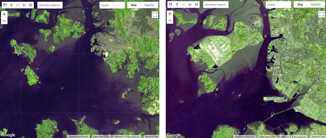
Change detection is the process of assessing how landscape conditions are changing by looking at differences in images acquired at different times. This can be used to quantify changes in forest cover—such as those following a volcanic eruption, logging activity, or wildfire—or when crops are harvested (Fig. F4.4.1). For example, using time-series change detection methods, Hansen et al. (2013) quantified annual changes in forest loss and regrowth. Change detection mapping is important for observing, monitoring, and quantifying changes in landscapes over time. Key questions that can be answered using these techniques include identifying whether a change has occurred, measuring the area or the spatial extent of the region undergoing change, characterizing the nature of the change, and measuring the pattern (configuration or composition) of the change (MacLeod and Congalton 1998).
a) b) c) d) |
Fig. F4.4.1 Before and after images of (a) the eruption of Mount St. Helens in Washington State, USA, in 1980 (before, July 10, 1979; after, September 5, 1980); (b) the Camp Fire in California, USA, in 2018 (before, October 7, 2018; after, March 16, 2019); (c) illegal gold mining in the Madre de Dios region of Peru (before, March 31, 2001; after, August 22, 2020); and (d) shoreline changes in Incheon, South Korea (before, May 29, 1981; after, March 11, 2020) |
Many change detection techniques use the same basic premise: that most changes on the landscape result in spectral values that differ between pre-event and post-event images. The challenge can be to separate the real changes of interest—those due to activities on the landscape—from noise in the spectral signal, which can be caused by seasonal variation and phenology, image misregistration, clouds and shadows, radiometric inconsistencies, variability in illumination (e.g., sun angle, sensor position), and atmospheric effects.
Activities that result in pronounced changes in radiance values for a sufficiently long time period are easier to detect using remote sensing change detection techniques than are subtle or short-lived changes in landscape conditions. Mapping challenges can arise if the change event is short-lived, as these are difficult to capture using satellite instruments that only observe a location every several days. Other types of changes occur so slowly or are so vast that they are not easily detected until they are observed using satellite images gathered over a sufficiently long interval of time. Subtle changes that occur slowly on the landscape may be better suited to more computationally demanding methods, such as time-series analysis. Kennedy et al. (2009) provides a nice overview of the concepts and tradeoffs involved when designing landscape monitoring approaches. Additional summaries of change detection methods and recent advances include Singh (1989), Coppin et al. (2004), Lu et al. (2004), and Woodcock et al. (2020).
For land cover changes that occur abruptly over large areas on the landscape and are long-lived, a simple two-date image differencing approach is suitable. Two-date image differencing techniques are long-established methods for identifying changes that produce easily interpretable results (Singh 1989). The process typically involves four steps: (1) image selection and preprocessing; (2) data transformation, such as calculating the difference between indices of interest (e.g., the Normalized Difference Vegetation Index (NDVI)) in the pre-event and post-event images; (3) classifying the differenced image(s) using thresholding or supervised classification techniques; and (4) evaluation.
Practicum
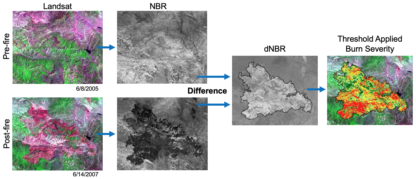
For the practicum, you will select pre-event and post-event image scenes and investigate the conditions in these images in a false-color composite display. Next, you will calculate the NBR index for each scene and create a difference image using the two NBR maps. Finally, you will apply a threshold to the difference image to establish categories of changed versus stable areas (Fig. F4.4.2).
Fig. F4.4.2 Change detection workflow for this practicum |
Section 1. Preparing Imagery
Before beginning a change detection workflow, image preprocessing is essential. The goal is to ensure that each pixel records the same type of measurement at the same location over time. These steps include multitemporal image registration and radiometric and atmospheric corrections, which are especially important. A lot of this work has been automated and already applied to the images that are available in Earth Engine. Image selection is also important. Selection considerations include finding images with low cloud cover and representing the same phenology (e.g., leaf-on or leaf-off).
The code in the block below accesses the USGS Landsat 8 Level 2, Collection 2, Tier 1 dataset and assigns it to the variable landsat8. To improve readability when working with the Landsat 8 ImageCollection, the code selects bands 2–7 and renames them to band names instead of band numbers.
var landsat8=ee.ImageCollection('LANDSAT/LC08/C02/T1_L2') |
Next, you will split the Landsat 8 ImageCollection into two collections, one for each time period, and apply some filtering and sorting to get an image for each of two time periods. In this example, we know there are few clouds for the months of the analysis; if you’re working in a different area, you may need to apply some cloud masking or mosaicing techniques (see Chap. F4.3).
The code below does several things. First, it creates a new geometry variable to filter the geographic bounds of the image collections. Next, it creates a new variable for the pre-event image by (1) filtering the collection by the date range of interest (e.g., June 2013), (2) filtering the collection by the geometry, (3) sorting by cloud cover so the first image will have the least cloud cover, and (4) getting the first image from the collection.
Now repeat the previous step, but assign it to a post-event image variable and change the filter date to a period after the pre-event image’s date range (e.g., June 2020).
var point=ee.Geometry.Point([-123.64, 42.96]); |
Section 2. Creating False-Color Composites
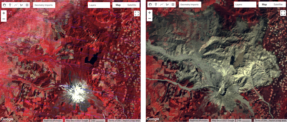
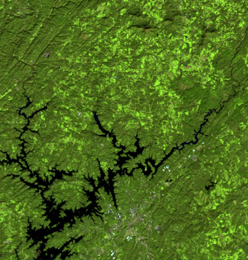
Before running any sort of change detection analysis, it is useful to first visualize your input images to get a sense of the landscape, visually inspect where changes might occur, and identify any problems in the inputs before moving further. As described in Chap. F1.1, false-color composites draw bands from multispectral sensors in the red, green, and blue channels in ways that are designed to illustrate contrast in imagery. Below, you will produce a false-color composite using SWIR-2 in the red channel, NIR in the green channel, and Red in the blue channel (Fig. F4.4.3).
Following the format in the code block below, first create a variable visParam to hold the display parameters, selecting the SWIR-2, NIR, and red bands, with values drawn that are between 7750 and 22200. Next, add the pre-event and post-event images to the map and click Run. Click and drag the opacity slider on the post-event image layer back and forth to view the changes between your two images.
var visParam={ |
Fig. F4.4.3 False-color composite using SWIR2, NIR, and red. Vegetation shows up vividly in the green channel due to vegetation being highly reflective in the NIR band. Shades of green can be indicative of vegetation density; water typically shows up as black to dark blue; and burned or barren areas show up as brown. |
Section 3. Calculating NBR
The next step is data transformation, such as calculating NBR. The advantage of using these techniques is that the data, along with the noise inherent in the data, have been reduced in order to simplify a comparison between two images. Image differencing is done by subtracting the spectral value of the first-date image from that of the second-date image, pixel by pixel (Fig. F4.4.2). Two-date image differencing can be used with a single band or with spectral indices, depending on the application. Identifying the correct band or index to identify change and finding the correct thresholds to classify it are critical to producing meaningful results. Working with indices known to highlight the land cover conditions before and after a change event of interest is a good starting point. For example, the Normalized Difference Water Index would be good for mapping water level changes during flooding events; the NBR is good at detecting soil brightness; and the NDVI can be used for tracking changes in vegetation (although this index does saturate quickly). In some cases, using derived band combinations that have been customized to represent the phenomenon of interest is suggested, such as using the Normalized Difference Fraction Index to monitor forest degradation (see Chap. A3.4).
Examine changes to the landscape caused by fires using NBR, which measures the severity of fires using the equation (NIR − SWIR) / (NIR + SWIR). These bands were chosen because they respond most strongly to the specific changes in forests caused by fire. This type of equation, a difference of variables divided by their sum, is referred to as a normalized difference equation (see Chap. F2.0). The resulting value will always fall between −1 and 1. NBR is useful for determining whether a fire recently occurred and caused damage to the vegetation, but it is not designed to detect other types of land cover changes especially well.
First, calculate the NBR for each time period using the built-in normalized difference function. For Landsat 8, be sure to utilize the NIR and SWIR2 bands to calculate NBR. Then, rename each image band with the built-in rename function.
// Calculate NBR. |
Code Checkpoint F44a. The book’s repository contains a script that shows what your code should look like at this point.
Section 4. Single Date Transformation
Next, we will examine the changes that have occurred, as seen when comparing two specific dates in time.
Subtract the pre-event image from the post-event image using the subtract function. Add the two-date change image to the map with the specialized Fabio Crameri batlow color ramp (Crameri et al. 2020). This color ramp is an example of a color combination specifically designed to be readable by colorblind and color-deficient viewers. Being cognizant of your cartographic choices is an important part of making a good change map.
// 2-date change. |
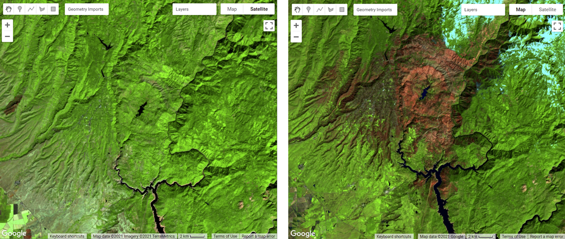
Question 1. Try to interpret the resulting image before reading on. What patterns of change can you identify? Can you find areas that look like vegetation loss or gain?
The color ramp has dark blues for the lowest values, greens and oranges in the midrange, and pink for the highest values. We used nbrPre subtracted from nbrPost to identify changes in each pixel. Since NBR values are higher when vegetation is present, areas that are negative in the change image will represent pixels that were higher in the nbrPre image than in the nbrPost image. Conversely, positive differences mean that an area gained vegetation (Fig. F4.4.4).
a) b) c) |
Fig. F4.4.4 (a) Two-date NBR difference; (b) pre-event image (June 2013) false-color composite; (c) post-event image (June 2020) false-color composite. In the change map (a), areas on the lower range of values (blue) depict areas where vegetation has been negatively affected, and areas on the higher range of values (pink) depict areas where there has been vegetation gain; the green/orange areas have experienced little change. In the pre-event and post-event images (b and c), the green areas indicate vegetation, while the brown regions are barren ground. |
Section 5. Classifying Change
Once the images have been transformed and differenced to highlight areas undergoing change, the next step is image classification into a thematic map consisting of stable and change classes. This can be done rather simply by thresholding the change layer, or by using classification techniques such as machine learning algorithms. One challenge of working with simple thresholding of the difference layer is knowing how to select a suitable threshold to partition changed areas from stable classes. On the other hand, classification techniques using machine learning algorithms partition the landscape using examples of reference data that you provide to train the classifier. This may or may not yield better results, but does require additional work to collect reference data and train the classifier. In the end, resources, timing, and the patterns of the phenomenon you are trying to map will determine which approach is suitable—or perhaps the activity you are trying to track requires something more advanced, such as a time-series approach that uses more than two dates of imagery.
For this chapter, we will classify our image into categories using a simple, manual thresholding method, meaning we will decide the optimal values for when a pixel will be considered change or no-change in the image. Finding the ideal value is a considerable task and will be unique to each use case and set of inputs (e.g., the threshold values for a SWIR2 single-band change would be different from the thresholds for NDVI). For a look at a more advanced method of thresholding, check out the thresholding methods in Chap. A2.3.
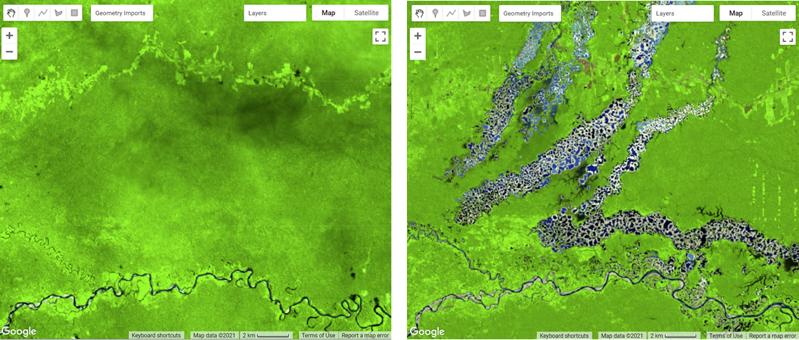
First, you will define two variables for the threshold values for gain and loss. Next, create a new image with a constant value of 0. This will be the basis of our classification. Reclassify the new image using the where function. Classify loss areas as 2 where the difference image is less than or equal to the loss threshold value. Reclassify gain areas to 1 where the difference image is greater than or equal to the gain threshold value. Finally, mask the image by itself and add the classified image to the map (Fig. F4.4.5). Note: It is not necessary to self-mask the image, and in many cases you might be just as interested in areas that did not change as you are in areas that did.
// Classify change |
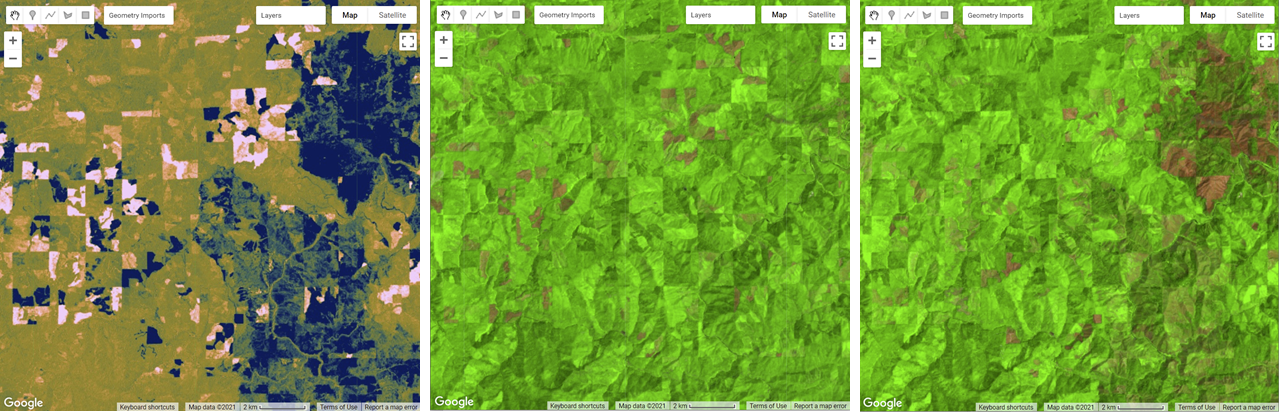
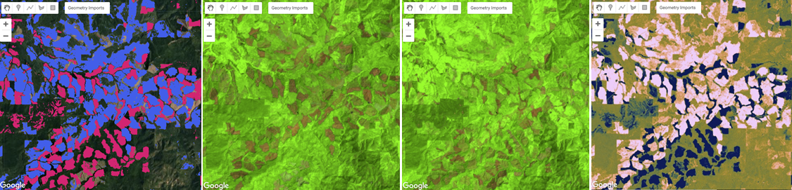
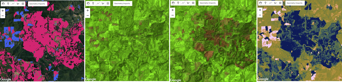
a) b) |
Fig. F4.4.5 (a) Change detection in timber forests of southern Oregon, including maps of the (left to right) pre-event false-color composite, post-event false-color composite, difference image, and classified change using NBR; (b) the same map types for an example of change caused by fire in southern Oregon. The false-color maps highlight vegetation in green and barren ground in brown. The difference images show NBR gain in pink to NBR loss in blue. The classified change images show NBR gain in blue and NBR loss in red. |
Chapters F4.5 through F4.9 present more-advanced change detection algorithms that go beyond differencing and thresholding between two images, instead allowing you to analyze changes indicated across several images as a time series.
Code Checkpoint F44b. The book’s repository contains a script that shows what your code should look like at this point.
Synthesis
Evaluating any maps you create, including change detection maps, is essential to determining whether the method you have selected is appropriate for informing land management and decision-making (Stehman and Czaplewski 1998), or whether you need to iterate on the mapping process to improve the final results. Maps generally, and change maps specifically, will always have errors. This is due to a suite of factors, such as the geometric registration between images, the calibration between images, the data resolution (e.g., temporal, spectral, radiometric) compared to the characteristics of the activity of interest, the complexity of the landscape of the study region (topography, atmospheric conditions, etc.), and the classification techniques employed (Lu et al. 2004). This means that similar studies can present different, sometimes controversial, conclusions about landscape dynamics (e.g., Cohen et al. 2017). In order to be useful for decision-making, a change detection mapping effort should provide the user with an understanding of the strengths and weaknesses of the product, such as by presenting omission and commission error rates. The quantification of classification quality is presented in Chap. F2.2.
Assignment 1. Try using a different index, such as NDVI or a Tasseled Cap Transformation, to run the change detection steps, and compare the results with those obtained from using NBR.
Assignment 2. Experiment with adjusting the thresholdLoss and thresholdGain values.
Assignment 3. Use what you have learned in the classification chapter (Chap. F2.1) to run a supervised classification on the difference layer (or layers, if you have created additional ones). Hint: To complete a supervised classification, you would need reference examples of both the stable and change classes of interest to train the classifier.
Assignment 4. Think about how things like clouds and cloud shadows could affect the results of change detection. What do you think the two-date differencing method would pick up for images in the same year in different seasons?
Conclusion
In this chapter, you learned how to make a change detection map using two-image differencing. The importance of visualizing changes in this way instead of using a post-classification comparison, where two classified maps are compared instead of two satellite images, is that it avoids multiplicative errors from the classifications and is better at observing more subtle changes in the landscape. You also learned that how you visualize your images and change maps—such as what band combinations and color ramps you select, and what threshold values you use for a classification map—has an impact on how easily and what types of changes can be seen.
Feedback
To review this chapter and make suggestions or note any problems, please go now to bit.ly/EEFA-review. You can find summary statistics from past reviews at bit.ly/EEFA-reviews-stats.
References
Cohen WB, Healey SP, Yang Z, et al (2017) How similar are forest disturbance maps derived from different Landsat time series algorithms? Forests 8:98. https://doi.org/10.3390/f8040098
Coppin P, Jonckheere I, Nackaerts K, et al (2004) Digital change detection methods in ecosystem monitoring: A review. Int J Remote Sens 25:1565–1596. https://doi.org/10.1080/0143116031000101675
Crameri F, Shephard GE, Heron PJ (2020) The misuse of colour in science communication. Nat Commun 11:1–10. https://doi.org/10.1038/s41467-020-19160-7
Fung T (1990) An assessment of TM imagery for land-cover change detection. IEEE Trans Geosci Remote Sens 28:681–684. https://doi.org/10.1109/TGRS.1990.572980
Hansen MC, Potapov PV, Moore R, et al (2013) High-resolution global maps of 21st-century forest cover change. Science 342:850–853. https://doi.org/10.1126/science.1244693
Kennedy RE, Townsend PA, Gross JE, et al (2009) Remote sensing change detection tools for natural resource managers: Understanding concepts and tradeoffs in the design of landscape monitoring projects. Remote Sens Environ 113:1382–1396. https://doi.org/10.1016/j.rse.2008.07.018
Lu D, Mausel P, Brondízio E, Moran E (2004) Change detection techniques. Int J Remote Sens 25:2365–2401. https://doi.org/10.1080/0143116031000139863
Macleod RD, Congalton RG (1998) A quantitative comparison of change-detection algorithms for monitoring eelgrass from remotely sensed data. Photogramm Eng Remote Sensing 64:207–216
Singh A (1989) Digital change detection techniques using remotely-sensed data. Int J Remote Sens 10:989–1003. https://doi.org/10.1080/01431168908903939
Stehman SV, Czaplewski RL (1998) Design and analysis for thematic map accuracy assessment: Fundamental principles. Remote Sens Environ 64:331–344. https://doi.org/10.1016/S0034-4257(98)00010-8
Woodcock CE, Loveland TR, Herold M, Bauer ME (2020) Transitioning from change detection to monitoring with remote sensing: A paradigm shift. Remote Sens Environ 238:111558. https://doi.org/10.1016/j.rse.2019.111558
References
Cloud-Based Remote Sensing with Google Earth Engine. (n.d.). CLOUD-BASED REMOTE SENSING WITH GOOGLE EARTH ENGINE. https://www.eefabook.org/
Cloud-Based Remote Sensing with Google Earth Engine. (2024). In Springer eBooks. https://doi.org/10.1007/978-3-031-26588-4