Terrestrial Applications part 2

Working With GPS and Weather Data

Cloud-Based Remote Sensing with Google Earth Engine

Fundamentals and Applications

Part A3: Terrestrial Applications

Earth’s terrestrial surface is analyzed regularly by satellites, in search of both change and stability. These are of great interest to a wide cross-section of Earth Engine users, and projects across large areas illustrate both the challenges and opportunities for life on Earth. Chapters in this Part illustrate the use of Earth Engine for disturbance, understanding long-term changes of rangelands, and creating optimum study sites.

Chapter A3.6: Working With GPS and Weather Data

Authors

Peder Engelstad, Daniel Carver, Nicholas E. Young

Overview

The purpose of this chapter is to demonstrate how to use Google Earth Engine as a means of associating remotely sensed data (weather observations) with open-source GPS point locations. These methods will provide a quick and easy way to access and analyze large amounts of information relative to your own research and efficiently move your data outside Earth Engine.

Learning Outcomes

Pairing values from remotely sensed data with uploaded data.
Exporting features from Earth Engine.

Helps if you know how to:

Import images and image collections, filter, and visualize (Part F1).
Exporting calculated data to tables with Tasks (Chap. F5.0).

Introduction to Theory

Knowing how animals interact with their environment is critical to understanding how to manage them. The choices animals make are influenced by basic survival needs (e.g., food, shelter, water) and dynamic factors such as local weather conditions. Without direct observation, it can be difficult to understand the relationship between animal movement and weather conditions.

In this chapter, we will explore information retrieved from a GPS collar worn by a cougar, and explore its relationship to daily temperature estimates from the Daymet climatological dataset available in Google Earth Engine. This will require us to bring an asset into Earth Engine, connect the weather values to the point locations, and bring those value-added data back out of Earth Engine for further analysis.

Github Code link for all tutorials

This code base is collection of codes that are freely available from different authors for google earth engine.

Github Source

Practicum

Section 1. GPS Location Data

Using GPS collars, Mahoney et al. (2017) tracked the movement of 2 cougars and 16 coyotes in central Utah. These data were used to understand some of the behavioral patterns of the individuals. These data have been freely shared with the broader research community and the public through Movebank, an online repository for animal movement datasets from across the globe. While some Movebank datasets list only the contact information of the authors, others (like those from the Mahoney study) allow you to display and download the information via an interactive web map.

We will pair the data on cougar movement with Daymet weather data. According to the Daymet website, the dataset “provides gridded estimates of daily weather parameters. Seven surface weather parameters are available at a daily time step, 1 km x 1 km spatial resolution, with a North American spatial extent allowing a rich resource of daily surface meteorology.”

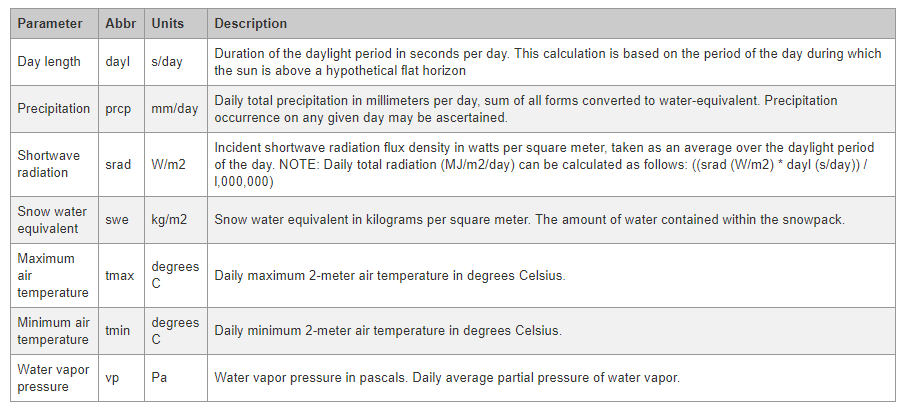
With data for every day at a 1 km2 spatial resolution, the Daymet data are a great resource for the temporal and spatial scale at which a cougar would interact with the landscape. There are seven measured values in total, allowing us to check multiple aspects of the weather to assess how it may be affecting behavior (Fig. A3.6.1).

Fig. A3.6.1 Metadata for Daymet imagery within Earth Engine

Section 2. Bringing Data into Earth Engine

In this chapter, we will discuss how to import assets into Earth Engine, extract values from a dataset, and export those values out of Earth Engine. The processes by which you can bring data into Earth Engine change frequently, so it is best to go directly to the documentation to view the latest updates.

Section 2.1. Bringing in an Asset

Using the following code, start a fresh script and import Mahoney’s cougar movement data from Movebank (which has already been uploaded for you in the assets of this book). Here, we will focus on a single animal (cougar ID F53). Because the original dataset was in csv format, it has been converted into a shapefile outside of GEE. During this process, it is important to note that data has been projected to the WGS 1984 (EPSG: 4326) coordinate reference system. Projecting to EPSG:4326 is recommended in Earth Engine to minimize the reprojection errors during the uploading process.

// Import the data and add it to the map and print.
var cougarF53=ee.FeatureCollection(
'projects/gee-book/assets/A3-6/cougarF53');

Map.centerObject(cougarF53, 10);

Map.addLayer(cougarF53,{}, 'cougar presence data');

print(cougarF53, 'cougar data');

You can use the Inspector tool to look at the attribute data associated with the new asset. With the points visualized, make a geometry feature that encompasses our area of interest by selecting the square geometry tool and drawing a box that encompasses the points (Fig. A3.6.2). We will use the geometry feature to filter our climate data.

Fig. A3.6.2 Draw a geometry feature around the points to spatially filter the climate data

Section 2.2. Defining Weather Variables

In this chapter, we are using Earth Engine as a means of associating remotely sensed data (i.e., our rasters) with our point locations. While the process is conceptually straightforward, it does take some work to accomplish. With our points loaded, the next step is to import the Daymet weather variables.

We are using the NASA-derived dataset Daymet V4 due to its 1 km2 spatial resolution and the fact that it measures the environmental variables we think might be related to cougar movement or behavior. We will import these variables by calling the unique ID of the dataset, filtering it to our bounding box geometry and the dates during which the data were collected.

// Call in image collection and filter.
var Daymet=ee.ImageCollection('NASA/ORNL/DAYMET_V4')
.filterDate('2014-02-11', '2014-11-02')
.filterBounds(geometry)
.map(function(image){
return image.clip(geometry);
});

print(Daymet, 'Daymet');

Fig. A3.6.3 A view of the structure of the Daymet V4 data from the print statement

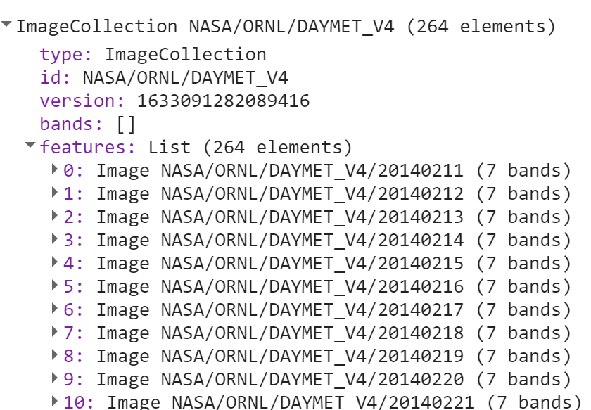
From the print statement (Fig. A3.6.3), we can see that this is an ImageCollection with 264 images (though your total number of images may be different, as the dataset changes over time). Each image has seven bands relating to specific weather measurements (see Fig. A3.6.1). Now that both datasets are loaded, we will associate the cougar occurrences data with the weather data.

Section 2.3. Extracting Values

With our points and imagery loaded, we can call a function to extract values from the underlying raster based on the known locations of the cougar. We will do this using the ee.Image.sampleRegions function. Search for the ee.Image.sampleRegions function under the Docs tab to familiarize yourself with the parameters it requires.

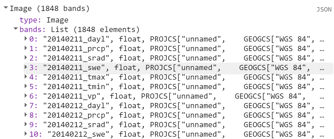
If we tried to call this function on the Daymet ImageCollection we would get an error, because ee.Image.sampleRegions is a function of an image. To get around this, we will convert the Daymet ImageCollection into a multiband image (Fig. A3.6.4). Each of the seven measurements for each day will become a specific band in our multiband image. This process will help us in the end, because each band is defined by the date it was collected and the variable it shows. We can use this information to determine which data connects to the positions of the cougar on a specific day.

It is important to note that, with many images in the ImageCollection, we are going to create a single image with a large number of bands. Because Earth Engine is good at data manipulations, it can handle this type of request.

// Convert to a multiband image.
var DaymetImage=Daymet.toBands();

print(DaymetImage, 'DaymetImage');

Fig. A3.6.4 A print statement showing the result of converting the Daymet ImageCollection into a multiband image

Now that we have a single multiband image, we can use the sampleRegions function to extract information across multiple dates at each of our GPS point locations (Fig. A3.6.5). There are three parameters of this function that should be considered:

Collection This is the vector dataset that the sampled data will be associated with.
Properties This defines which columns of the vector dataset will remain. In this case, we want to keep the ID column, because that is what we will use to join this dataset back to the original outside of Earth Engine.
Scale This refers to the spatial resolution of the dataset. The scale parameter should always match the spatial resolution of your raster data. If you are not sure what the resolution of a raster is, you can search for the dataset using the search bar and locate that information in the documentation. (If you want to get the number for use in code, the nominalScale function, as described in Chap. F1.3, can extract it from an image.)

// Call the sample regions function.
var samples=DaymetImage.sampleRegions({
collection: cougarF53,
properties: ['id'],
scale: 1000
});

print(samples, 'samples');

Fig. A3.6.5 The print statement from the sampleRegions function showing that our GPS point locations now have weather measurements associated with them

Code Checkpoint A36a. The book’s repository contains a script that shows what your code should look like at this point.

Section 2.4. Exporting

Exporting Points

We now have a series of daily weather data associated with the known locations of the cougar known as F53. While we could work more with these data in Earth Engine, it will be easy to bring them into R, Python, or Excel for further analysis. There are a few options to define where the exported data will be created. Generally speaking, saving the data to a Google Drive account provides an easy way to access the data with another program. Here, we will use a dictionary, denoted by the curly brackets {}, to define the parameters of the Export.table.toDrive function.

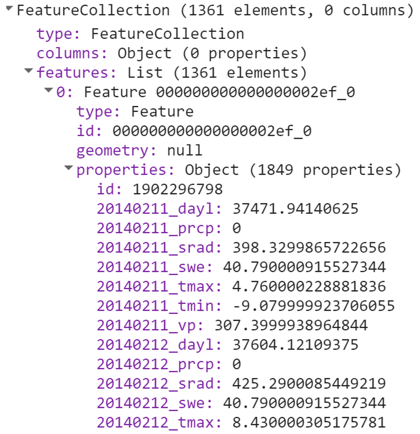
We would have preferred to export to create a shapefile, but a shapefile can contain only 255 columns. The samples variable has 1361 columns, so we will export the data as a CSV file.

// Export value added data to your Google Drive.
Export.table.toDrive({
collection: samples,
description: 'cougarDaymetToDriveExample',
fileFormat: 'csv'
});

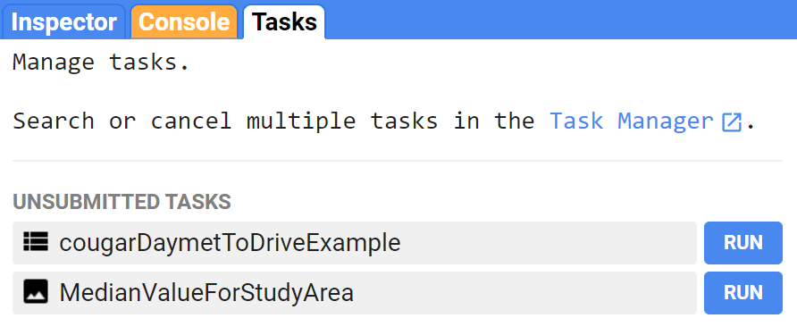
When you export something, the Tasks panel will light up. To run the task, click the Run button (Fig. A3.6.6).

Fig. A3.6.6 An example of the Tasks bar once a script with an export function has been run

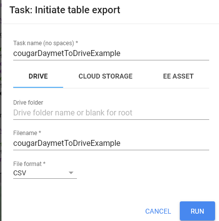
When you click the Run button, the pop-up shown in Fig. A3.6.7 will appear. This allows you to edit the details of the export.

Fig. A3.6.7 An example of the user-defined parameters present when exporting a feature from Earth Engine

Exporting a Raster

While working with these spatial data, you may have realized that a raster showing the median values over the time period when data were collected on the cougar could be useful information to have. To do this, we will apply a median reducer function to the Daymet ImageCollection to generate a median value for each parameter in each cell. As with the tabular data, we will export this multiband image to Google Drive. Once we convert the ImageCollection to an image using the median function, we can clip it to the geometry feature object. This feature will be exported as a multiband raster.

// Apply a median reducer to the dataset.
var daymet1=Daymet
.median()
.clip(geometry);

print(daymet1);

// Export the image to drive.
Export.image.toDrive({
image: daymet1,
description: 'MedianValueForStudyArea',
scale: 1000,
region: geometry,
maxPixels: 1e9
});

In Earth Engine, there are many options for exporting images. One of the most important options when exporting data is the maxPixels parameter. Generally speaking, Earth Engine will not allow you to export a raster with more than 109 pixels. With the maxPixels parameter, you can bump this up to around 1012 pixels per image. If you are exporting data for an area larger than 1012 pixels, you will need to be creative about how to get the information out of Earth Engine. Sometimes this involves splitting the image into smaller pieces (as described in Chap. F6.2), or even reevaluating the usefulness of such a large image outside of Earth Engine.

Code Checkpoint A36b. The book’s repository contains a script that shows what your code should look like at this point.

Question 1. With the maxPixels count set to 1e9, what square area would you expect to be able to export for imagery with 1000, 250, 30, 10 m cell size? Determine how this area measure changes when using 1012 pixels for one of the cell sizes to determine the percent increase.

Question 2. We selected all available variables from the Daymet collection. What specific bands from Daymet might be most relevant to cougars? How would you edit the code to select just one or a few bands?

Question 3. When we extracted the raster data, we set the scale parameter to 1000 to match the known spatial resolution of the Daymet dataset. Would it be reasonable to change that scale parameter to 500 to get final resolution data? What does Earth Engine tell you when you attempt to change the scale of an export?

Synthesis

Assignment 1. Utilize the chapter’s script with a different dataset to process tracking information from a different animal from Movebank or another occurrence database of your choice (e.g., GBIF.org). Evaluate whether the temperature ranges between the two animals are different and make a hypothesis about why this might be.

Conclusion

While Google Earth Engine can be used for planetary-scale analyses, it is also an effective resource for quickly accessing and analyzing large amounts of information across time at a scale relative to your own data. The method presented in this chapter is a great way to add value to your own research. Here, we worked with weather data, but that is by no means the only option. You can connect your data to many other datasets within Earth Engine. It is up to you to explore and find what is relevant to your work.

Feedback

To review this chapter and make suggestions or note any problems, please go now to bit.ly/EEFA-review. You can find summary statistics from past reviews at bit.ly/EEFA-reviews-stats.

References

Cloud-Based Remote Sensing with Google Earth Engine. (n.d.). CLOUD-BASED REMOTE SENSING WITH GOOGLE EARTH ENGINE. https://www.eefabook.org/

Cloud-Based Remote Sensing with Google Earth Engine. (2024). In Springer eBooks. https://doi.org/10.1007/978-3-031-26588-4

Mahoney PJ, Young JK (2017) Uncovering behavioural states from animal activity and site fidelity patterns. Methods Ecol Evol 8:174–183. https://doi.org/10.1111/2041-210X.12658