Terrestrial Applications part 2

Conservation II Assessing Agricultural Intensification Near Protected Areas

Cloud-Based Remote Sensing with Google Earth Engine

Fundamentals and Applications

Part A3: Terrestrial Applications

Earth’s terrestrial surface is analyzed regularly by satellites, in search of both change and stability. These are of great interest to a wide cross-section of Earth Engine users, and projects across large areas illustrate both the challenges and opportunities for life on Earth. Chapters in this Part illustrate the use of Earth Engine for disturbance, understanding long-term changes of rangelands, and creating optimum study sites.

Chapter A3.10: Conservation II - Assessing Agricultural Intensification Near Protected Areas

Authors

Pradeep Koulgi and MD Madhusudan

Overview

Protected Areas (PAs) in many densely populated tropical regions are often small in area, and are enormously influenced by the broader production landscapes in which they are found. Changes in the agricultural matrix surrounding a PA can have a profound impact on the PA’s wildlife and on neighboring resident human communities. In this chapter, we will examine greening trend changes in the exteriors of 186 PAs in Western India from 2000 to 2021 using MODIS Terra vegetation indices, a Sen’s slope linear trend estimator, and other summary techniques available in Earth Engine. We will use these techniques to investigate how these greening trends are distributed in relation to the precipitation regimes of a given PA site.

Learning Outcomes

Computing a metric of a monotonic trend (Sen’s slope) in dry-season pixel greenness for each pixel.
Inferring the nature and intensity of change in agricultural practice based on the trend metric.
Exploring the relationship between changes in vegetation greenness and ecosystem type as determined by average annual precipitation.

Helps if you know how to:

Import images and image collections, filter, and visualize (Part F1).
Perform basic image analysis: select bands, compute indices, create masks (Part F2).
Calculate and interpret vegetation indices (Chap. F2.0)
Use reducers to implement linear regression between image bands (Chap. F3.0).
Write a function and map it over an ImageCollection (Chap. F4.0).
Map an annual reducer across multiple years (Chap. F4.0, Chap. F4.1).
Write a function and map it over a collection (Chap. F4.0).
Conduct basic vector analyses: vectorizing and buffering (Part F5).
Write a function and map it over a FeatureCollection (Chap. F5.1, Chap. F5.2).

Github Code link for all tutorials

This code base is collection of codes that are freely available from different authors for google earth engine.

Github Source

Introduction to Theory

In many regions of the densely populated tropics, Protected Areas (PAs) are often small, and their interfaces with production landscapes are sharp. As a result, changes in the agriculture surrounding a PA can have a profound impact on the PA’s wildlife, as well as on their interactions with local human communities. For example, across India’s Gangetic Plains, increased crop irrigation via groundwater exploitation has enabled its traditional rainfed agriculture with long fallow periods and annual crops (cereals, legumes, and oilseeds) to be to be replaced by year-round agriculture (Chen et al 2019, Maina et al 2022). This intensification can have subtle yet significant changes in the landscape in terms of spatial regimes of primary productivity, and to wildlife in terms of both dietary and habitat resources. These changes, in turn, can influence wildlife interactions with people (Kumar et al. 2018).

In this chapter, we describe greening trends in vegetation in the exteriors of PAs in Western India, and ask how these greening trends are distributed in relation to the precipitation regimes of a given PA site. Based on our experience and our reading of literature pertaining to wildlife in India, we hypothesize that as crop irrigation via groundwater extraction increases, farming in the moisture-limited semi-arid tracts of India becomes more independent of seasonal differences, and their constituent habitats become structurally more complex. These changes could help create novel anthropogenic habitats that can be accessed by adaptable wildlife species living in PAs, such as leopards and elephants (Athreya and Ghoshal 2010, Odden et al. 2014). While such changes to habitat structure and resource availability could improve functional connectivity between PAs (e.g., Rodrigues et al. 2022), intensification can also lead to a greater overlap between humans and wildlife, possibly leading to greater conflict over crops and livestock (Kumar et al. 2018). The potential trade-offs involved between conservation and conflict imply that it is crucial to assess and map land use changes around PAs over time, and eventually to relate this to changes in wildlife distribution and behavior, for which this chapter provides a framework.

Practicum

Section 1. Initializing Parameters

The Normalized Difference Vegetation Index (NDVI) estimates vegetation greenness; the MODIS Terra vegetation indices products, MOD13Q1.006, provides historical 16-day composites of it at a global span and 250 m per pixel resolution. This dataset is used here to estimate a monotonic trend in annual changes of dry-season vegetation greenness around a set of PAs in India. Various parameters used in the script are initialized first.

Section 1.1 Annual dry-season Maximum NDVI Calculation

The MODIS vegetation indices dataset MOD13Q1.006 is initialized, along with the NDVI band name and relevant scale values. The dataset starts from the year 2000 and extends to the present. For this analysis, we use data from 2000 to 2021 as the sequence of full years the data are available for. The annual dry season in much of India occurs over three to five months, starting roughly in January. Here, a period of 90 days (spanning January through March) starting on the first day of each year is taken to be the dry season. Convenient names are chosen for bands holding NDVI and time values for regression analysis.

var modis_veg=ee.ImageCollection('MODIS/006/MOD13Q1');
var ndviBandName='NDVI';
var ndviValuesScaling=0.0001;
var modisVegScale=250; // meters
var maxNDVIBandname='max_dryseason_ndvi';
var yearTimestampBandname='year';
var years=ee.List.sequence(2000, 2021, 1);
var drySeasonStart_doy=1;
var drySeasonEnd_doy=90;

Section 1.2 Boundaries of PAs of Interest

In the code below, a set of PAs in the western part of India is identified for study. This collection of PAs in the western belt of India spans a wide range of rainfall regimes, from very moist areas in the southern Western Ghats to very arid regions in the Thar Desert of Rajasthan in the north, with diverse rainfall regimes in between. This belt is home to a diverse array of forests and savanna ecosystems, ranging from moist ecosystems to semi-arid and arid ecosystems. The landscapes in this belt also have a complex, diverse intervening matrix of natural and intensively human-utilized lands making up wildlife corridors. The size of the buffer area around each PA is also defined.

var paBoundaries=ee.FeatureCollection(
'projects/gee-book/assets/A3-10/IndiaMainlandPAs');
var boundaryBufferWidth=5000; // meters
var bufferingMaxError=30; // meters
// Choose PAs in only the western states
var western_states=[
'Rajasthan', 'Gujarat', 'Madhya Pradesh',
'Maharashtra', 'Goa', 'Karnataka', 'Kerala'
];
var western_pas=paBoundaries
.filter(ee.Filter.inList('STATE', western_states));

Section 1.3 Regression Analysis

The Sen’s slope linear trend estimator (Sen, 1968) is a non-parametric estimator useful for monotonic trend estimation applications using remotely sensed indices. Its suitability for applications with remotely sensed indices comes from a key difference when compared to linear regression using the least squares estimator: while linear regression assumes that the regression residuals are normally distributed, Sen's slope estimator makes no such assumptions about the statistical structure of the data it is being applied on. The reducer for this Sen’s slope regression is built into the Earth Engine API, and in the code below its x and y variables are initialized.

var regressionReducer=ee.Reducer.sensSlope();
var regressionX=yearTimestampBandname;
var regressionY=maxNDVIBandname;

Section 1.4 Surface Water Layer to Mask Water Pixels from Assessment

NDVI values of pixels spanning water bodies tend to be highly noisy and can mislead trend analyses. Masking out all pixels that were ever water during the period of interest can mitigate this problem. The European Union’s Joint Research Centre mapped monthly surface water from 1984 to 2021, including the maximum water extent detected during the period.

// Selects pixels where water has ever been detected between 1984 and 2021
var surfaceWaterExtent=ee.Image('JRC/GSW1_3/GlobalSurfaceWater')
.select('max_extent');

Section 1.5 Average Annual Precipitation Layer

To relate the estimated trends in vegetation greenness to rainfall regime, we use WorldClim’s estimated long-term average annual precipitation data.

var rainfall=ee.Image('WORLDCLIM/V1/BIO').select('bio12');

Section 1.6 Visualization and Saving Parameters

The estimated metric of change in vegetation greenness can be visualized as a raster on the map. Additionally, the relationship between changes in vegetation greenness and precipitation around each PA can be charted using a scatter plot. The visualization parameters for these are defined.

var regressionResultVisParams={
min: -3,
max: 3,
palette: ['ff8202', 'ffffff', '356e02']
};
var regressionSummaryChartingOptions={
title: 'Yearly change in dry-season vegetation greenness ' +
'in PA buffers in relation to average annual rainfall',
hAxis:{
title: 'Annual Precipitation'
},
vAxis:{
title: 'Median % yearly change in vegetation greenness ' +
'in 5 km buffer'
},
series:{
0:{
visibleInLegend: false
}
},
};

Code Checkpoint A310a. The book’s repository contains a script that shows what your code should look like at this point.

Section 2. Raster Processing for Change Analysis

The 16-day composite NDVI rasters are filtered, processed, and reduced according to parameters appropriately defined and initialized above to generate a raster of percentage annual change in greenness as a metric for vegetation change. A summary of this for each PA buffer is also calculated. Finally, these results are visualized.

Section 2.1 Annual Dry-season Maxima of NDVI

The source MODIS vegetation indices dataset is first filtered to the dry-season days for all years and the NDVI band selected. From this ImageCollection containing only dry-season observations for each year, maximum dry-season NDVI is calculated. This represents the vegetation at its greenest condition within the dry season each year. The maximum NDVI is the least likely to be influenced by episodic changes, such as fires that occur during this dry period. An image band containing the year value is also created and combined with the maximum NDVI, in preparation for time versus NDVI regression analysis in the next step. This is accomplished through defining a function annualDrySeasonMaximumNDVIAndTime to do this for each year, and then mapping that function over all the years in our period of interest.

function annualDrySeasonMaximumNDVIAndTime(y){
// Convert year y to a date object
var yDate=ee.Date.fromYMD(y, 1, 1);
// Calculate max NDVI for year y
var yMaxNdvi=drySeasonNdviColl
// Filter to year y
.filter(ee.Filter.date(yDate, yDate.advance(1, 'year')))
// Compute max value
.max()
// Apply appropriate scale, as per the dataset's
// technical description for NDVI band.
.multiply(ndviValuesScaling)
// rename the band to be more comprehensible
.rename(maxNDVIBandname);
// Create an image with constant value y, to be used in regression. Name it something comprehensible.
// Name it something comprehensible.
var yTime=ee.Image.constant(y).int().rename(
yearTimestampBandname);
// Combine the two images into a single 2-band image, and return
return ee.Image.cat([yMaxNdvi, yTime]).set('year', y);
}

// Create a collection of annual dry season maxima
// for the years of interest. Select the NDVI band and
// filter to the collection of dry season observations.
var drySeasonNdviColl=modis_veg.select([ndviBandName])
.filter(ee.Filter.calendarRange(drySeasonStart_doy,
drySeasonEnd_doy, 'day_of_year'));
// For each year of interest, calculate the NDVI maxima and create a corresponding time band
var dryseason_coll=ee.ImageCollection.fromImages(
years.map(annualDrySeasonMaximumNDVIAndTime)
);

Section 2.2 Annual Regression to Estimate Average Yearly Change in Greenness

The dry-season maximum NDVI collection with time band is reduced with a Sen’s slope regression reducer to estimate the linear rate of change of dry-season maximum greenness for the years from 2000 to 2021. Be sure to use the select operation to select the x and y variables for regression, in that order, as expected by the ee.Reducer.sensSlope. The resulting image will have a slope and an offset band, which are the slope and y-intercept of the trend estimation, respectively.

The values in the slope band are the pixel-wise annual rate of change in maximum dry-season NDVI values. The magnitude of these values signifies the intensity of change over the years, and their sign indicates whether the change manifested as greening (positive sign) or browning (negative sign) of the vegetation.

var ss=dryseason_coll.select([regressionX, regressionY]).reduce(
regressionReducer);

// Mask surface water from vegetation change image
var ss=ss.updateMask(surfaceWaterExtent.eq(0));

Section 2.3 Summarize Estimates of Change in Buffer Regions of PAs of Interest

In order to investigate the vegetation greening and browning changes within the buffer areas of our PAs of interest, buffer regions have to be defined. This can be done by computing the geometry 'difference” between the buffered version of each PA and the PA itself. A function extractBufferRegion is defined to perform this for each PA feature, and that function is mapped over the feature collection with boundaries of all the PAs of interest.

function extractBufferRegion(pa) {
//reduce vertices in PA boundary
pa=pa.simplify({
maxError: 100
});
// Extend boundary into its buffer
var withBuffer=pa.buffer(boundaryBufferWidth,
bufferingMaxError);
// Compute the buffer-only region by "subtracting" boundary with buffer from boundary
// Subtracting the whole set of boundaries eliminates inclusion of forests from adjacent PAs into buffers.
var bufferOnly=withBuffer.difference(paBoundaries.geometry());

return bufferOnly;
}

// Create buffer regions of PAs
var pa_buff=western_pas.map(extractBufferRegion);

The greenness condition of vegetation in the dry season is inherently variable in large diverse landscapes like around the PAs of choice here, and it depends strongly on the type of vegetation itself, such as deciduous or evergreen tree cover, grasslands, shrublands, and croplands. In order to take this inherent variability into account, the raw rate of change value can be converted into a percent rate of change by normalizing the change value against a baseline value. Here, the maximum year 2000 dry-season NDVI is used as the baseline in each pixel. The slope values are normalized using this baseline and converted to percent values. This can be visualized on the map.

In order to understand the overall picture at a PA buffer-region level, the median of percent rate of vegetation change is calculated for every PA buffer. And to relate this to the amount of rainfall in a buffer region, the corresponding median of average annual rainfall over the region is also calculated. These can be visualized in a chart.

// Normalize the metric of NDVI change to a baseline (dry-season max NDVI in the very first year)
var baselineNdvi=dryseason_coll.select([maxNDVIBandname]).filter(ee
.Filter.eq('year', years.getNumber(0))).first();
var stats=ss.select('slope').divide(baselineNdvi).multiply(100)
.rename('vegchange');

// Combine it with average annual rainfall data
stats=stats.addBands(rainfall.rename('rainfall'));

// Calculate mean of change metric over buffer regions of each PA of interest
var paBufferwiseMedianChange=stats.reduceRegions({
collection: pa_buff,
reducer: ee.Reducer.median(),
scale: 1000,
tileScale: 16
});

Code Checkpoint A310b. The book’s repository contains a script that shows what your code should look like at this point.

Section 3. Visualizing Results

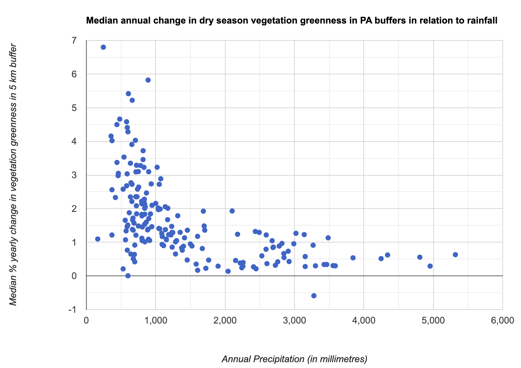
The degree of vegetation change, with a chosen palette, is visualized as a map (Fig. A3.10.1), and the PA buffer-wise median value is charted as a scatter plot (Fig. A3.10.2). In the map, green color suggests significant vegetation greening, brown color suggests significant vegetation browning, and white color suggests no detectable change, as chosen in the palette. The vegetation in large areas in the surroundings of Nauradehi Wildlife Sanctuary, as highlighted by Fig. A3.10.1, appear to have experienced greening or no detectable change. PA buffer-wise summaries showing moderate to high positive values indicate that, across the buffers of the PAs, there appears to have been a greater extent of greening, rather than browning, of vegetation cover.

The degree of vegetation change is also arranged by amount of rainfall in a chart, to visualize how buffer regions of PAs in moist regions fare relative to those in arid regions.

var medianChangeChart=ui.Chart.feature.byFeature({
features: paBufferwiseMedianChange,
xProperty: 'rainfall',
yProperties: ['vegchange']
}).setOptions(regressionSummaryChartingOptions).setChartType(
'ScatterChart');
print(medianChangeChart);

Map.centerObject(western_pas, 9);
Map.setCenter(79.2205, 23.3991, 9);
Map.setOptions('SATELLITE');
Map.addLayer(stats.select('vegchange').clipToCollection(pa_buff),
regressionResultVisParams, 'yearly % change');
Map.addLayer(western_pas,{}, 'Western PAs');

Code Checkpoint A310c. The book’s repository contains a script that shows what your code should look like at this point.

Fig. A3.10.1 Map of percent vegetation greenness change for 2000–2021 in a 5-km buffer area around Nauradehi Wildlife Sanctuary (polygon in black shade), India. Note the relative absence of vegetation browning.

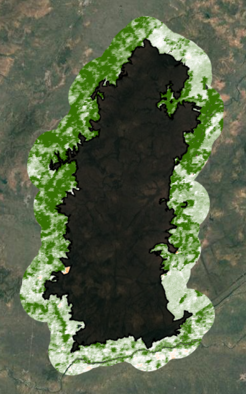
Fig. A3.10.2 Median yearly percent change in vegetation greenness observed in 5-km exterior buffers of PAs in India (N=186), arranged along a precipitation gradient. Greening is denoted by a positive percent change in Sen’s slope of dry-season maximum NDVI between 2000 and 2021. The greatest greening extent (>2%) is observed in PAs that fall in the semi-arid zone (annual precipitation ≤ 1000 mm).

Question 1. Create a map of percent vegetation greenness change for a different PA than the one shown in Fig. A3.10.1. How does it compare with the map made for Nauradehi Wildlife Sanctuary?

Question 2. We used MODIS Terra vegetation indices for our greening trend analysis in the previous example. Can you alter the analysis to calculate an NDVI time series from Landsat imagery for one PA? How do you think the results would change with Landsat’s 30 m spatial resolution instead of 250 m from MODIS?

Question 3. Can you repeat this analysis, dividing the time period of 21 years into two approximate halves, and try to determine whether the slope of vegetation greening observed has been similar across the two periods, or whether greening has accelerated or decelerated between the two time periods?

Synthesis

Assignment 1. In this chapter, you learned how to estimate greening trends surrounding PAs in Western India, a densely populated tropical region. In your opinion, how generalizable are these observed patterns across space and time?

Assignment 2. Perform this same PA analysis in another region in India. Then, perform the same analysis in a tropical region in another part of the world. How do the results compare with ours from Western India?

Conclusion

In this chapter, we estimated greening trends in Western India PAs using MODIS Terra vegetation indices, Sen’s slope, and reducer functions. We demonstrated that the immediate exterior buffers of most PAs (184 out of 186) show a positive—i.e., greening—trend in their vegetation cover over the two-decade time frame between 2000 and 2021. Note, however, that in this example we do not estimate the significance level of the greening trend values modeled in our analyses. While there is considerable variation in the greening extent seen across these PA buffers, we do see clearly that PAs that fall within the semi-arid zone (annual precipitation ≤ 1000 mm) seem to show the greatest extent of greening (Fig. A3.10.2). Such a change in the land cover characteristics of the matrix surrounding PAs in the semi-arid zone suggests that they are more likely to be sites where the distribution of wildlife, especially of more adaptable species, could show expansion into the agricultural landscape beyond PA boundaries, as well as greater rates of conflict with humans over crops and livestock. Corroborating this, of course, requires ground survey data on wildlife, which were unavailable in this example.

Feedback

To review this chapter and make suggestions or note any problems, please go now to bit.ly/EEFA-review. You can find summary statistics from past reviews at bit.ly/EEFA-reviews-stats.

References

Cloud-Based Remote Sensing with Google Earth Engine. (n.d.). CLOUD-BASED REMOTE SENSING WITH GOOGLE EARTH ENGINE. https://www.eefabook.org/

Cloud-Based Remote Sensing with Google Earth Engine. (2024). In Springer eBooks. https://doi.org/10.1007/978-3-031-26588-4

Chen C, Park T, Wang X, et al (2019) China and India lead in greening of the world through land-use management. Nat Sustain 2:122–129. https://doi.org/10.1038/s41893-019-0220-7

Kumar MA, Vijayakrishnan S, Singh M (2018) Whose habitat is it anyway? Role of natural and anthropogenic habitats in conservation of charismatic species. Trop Conserv Sci 11:1940082918788451. https://doi.org/10.1177/1940082918788451

Lenin J (2010) Sugarcane leopards. In: Current Conservation, Special: Wildlife-Human Conflict. https://www.currentconservation.org/sugarcane-leopards/

Maina FZ, Kumar SV, Albergel C, Mahanama SP (2022) Warming, increase in precipitation, and irrigation enhance greening in High Mountain Asia. Commun Earth Environ 3:1–8. https://doi.org/10.1038/s43247-022-00374-0

Odden M, Athreya V, Rattan S, Linnell JDC (2014) Adaptable neighbours: Movement patterns of GPS-collared leopards in human dominated landscapes in India. PLoS One 9:e112044. https://doi.org/10.1371/journal.pone.0112044

Rodrigues RG, Srivathsa A, Vasudev D (2022) Dog in the matrix: Envisioning countrywide connectivity conservation for an endangered carnivore. J Appl Ecol 59:223–237. https://doi.org/10.1111/1365-2664.14048

Sen PK (1968) Estimates of the regression coefficient based on Kendall’s tau. J Am Stat Assoc 63:1379–1389. https://doi.org/10.1080/01621459.1968.10480934