Cloud-Based Remote Sensing with Google Earth Engine
Fundamentals and Applications

Part F6: Advanced Topics
Although you now know the most basic fundamentals of Earth Engine, there is still much more that can be done. The Part presents some advanced topics that can help expand your skill set for doing larger and more complex projects. These include tools for sharing code among users, scaling up with efficient project design, creating apps for non-expert users, and combining R with other information processing platforms.
Chapter F6.4: Combining R and Earth Engine
Authors
Cesar Aybar, David Montero, Antony Barja, Fernando Herrera, Andrea Gonzales, and Wendy Espinoza
Overview
The purpose of this chapter is to introduce rgee, a non-official API for Earth Engine. You will explore the main features available in rgee and how to set up an environment that integrates rgee with third-party R and Python packages. After this chapter, you will be able to combine R, Python, and JavaScript in the same workflow.
Learning Outcomes
- Becoming familiar with rgee, the Earth Engine R API interface.
- Integrating rgee with other R packages.
- Displaying interactive maps.
- Integrating Python and R packages using reticulate.
- Combining Earth Engine JavaScript and Python APIs with R.
Assumes you know how to:
- Install the Python environment (Chap. F6.3).
- Use the require function to load code from existing modules (Chap. F6.1).
- Use the basic functions and logic of Python.
- Configure an environment variable and use .Renviron files.
- Create Python virtual environments.
Github Code link for all tutorials
This code base is collection of codes that are freely available from different authors for google earth engine.
Introduction to Theory
R is a popular programming language established in statistical science with large support in reproducible research, geospatial analysis, data visualization, and much more. To get started with R, you will need to satisfy some extra software requirements. First, install an up-to-date R version (at least 4.0) in your work environment. The installation procedure will vary depending on your operating system (i.e., Windows, Mac, or Linux). Hands-On Programming with R (Garrett Grolemund 2014, Appendix A) explains step by step how to proceed. We strongly recommend that Windows users install Rtools to avoid compiling external static libraries.
If you are new to R, a good starting point is the book Geocomputation with R (Lovelace et al. 2019) or Spatial Data Science with Application in R (Pebesma and Bivand 2021). In addition, we recommend using an integrated development environment (e.g., Rstudio) or a code editor (e.g., Visual Studio Code) to create a suitable setting to display and interact with R objects.
The following R packages must be installed (find more information in the R manual) in order to go through the practicum section.
# Use install.packages to install R packages from the CRAN repository. |
Earth Engine officially supports client libraries only for the JavaScript and Python programming languages. While the Earth Engine Code Editor offers a convenient environment for rapid prototyping in JavaScript, the lack of a mechanism for integration with local environments makes the development of complex scripts tricky. On the other hand, the Python client library offers much versatility, enabling support for third-party packages. However, not all Earth and environmental scientists code in Python. Hence, a significant number of professionals are not members of the Earth Engine community. In the R ecosystem, rgee (Aybar et al. 2020) tries to fill this gap by wrapping the Earth Engine Python API via reticulate (Kevin Ushey et al. 2021). The rgee package extends and supports all the Earth Engine classes, modules, and functions, working as fast as the other APIs.
Fig. F6.4.1 A simplified diagram of rgee functionality |
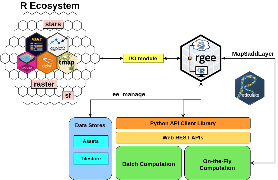
Figure F6.4.1 illustrates how rgee bridges the Earth Engine platform with the R ecosystem. When an Earth Engine request is created in R, rgee transforms this piece of code into Python. Next, the Earth Engine Python API converts the Python code into JSON. Finally, the JSON file request is received by the server through a Web REST API. Users could get the response using the getInfo method by following the same path in reverse.
Practicum
Section 1. Installing rgee
To run, rgee needs a Python environment with two packages: NumPy and earthengine-api. Because instructions change frequently, installation is explained at the following checkpoint:
Code Checkpoint F64a. The book’s repository contains information about setting up the rgee environment.
After installing both the R and Python requirements, you can now initialize your Earth Engine account from within R. Consider that R, in contrast to Javascript and Python, supports three distinct Google APIs: Earth Engine, Google Drive, and Google Cloud Storage (GCS).
The Google Drive and GCS APIs will allow you to transfer your Earth Engine completed task exports to a local environment automatically. In these practice sessions, we will use only the Earth Engine and Google Drive APIs. Users that are interested in GCS can look up and explore the GCS vignette. To initialize your Earth Engine account alongside Google Drive, use the following commands.
# Initialize just Earth Engine |
If the Google account is verified and the permission is granted, you will be directed to an authentication token. Copy and paste this token into your R console. Consider that the GCS API requires setting up credentials manually; look up and explore the rgee vignette for more information. The verification step is only required once; after that, rgee saves the credentials in your system.
Code Checkpoint F64b. The book’s repository contains information about what your code should look like at this point.
Section 2. Creating a 3D Population Density Map with rgee and rayshader
First, import the rgee, rayshader, and raster packages.
library(rayshader) |
Initialize the Earth Engine and Google Drive APIs using ee_Initialize. Both credentials must come from the same Google account.
ee_Initialize(drive=TRUE) |
Then, we will access the WorldPop Global Project Population Data dataset. In rgee, the Earth Engine spatial classes (ee$Image, ee$ImageCollection, and ee$FeatureCollection) have a special attribute called Dataset. Users can use it along with autocompletion to quickly find the desired dataset.
collections <- ee$ImageCollection$Dataset |
If you need more information about the Dataset, use ee_utils_dataset_display to go to the official documentation in the Earth Engine Data Catalog.
population_data %>% ee_utils_dataset_display() |
The rgee package provides various built-in functions to retrieve data from Earth Engine (Aybar et al. 2020). In this example, we use ee_as_raster, which automatically converts an ee$Image (server object) into a RasterLayer (local object).
sa_extent <- ee$Geometry$Rectangle( |
Now, turn a RasterLayer into a matrix suitable for rayshader.
pop_matrix <- raster_to_matrix(population_data_ly_local) |
Next, modify the matrix population density values, adding:
- Texture, based on five colors (lightcolor, shadowcolor, leftcolor, rightcolor, and centercolor; see rayshader::create_texture documentation)
- Color and shadows (rayshader::sphere_shade)
pop_matrix %>% |
Lastly, define a title and subtitle for the plot. Use rayshader::render_snapshot to export the final results (Fig. F6.4.2).
text <- paste0( |
Fig. F6.4.2 3D population density map of South America |

Code Checkpoint F64c. The book’s repository contains information about what your code should look like at this point.
Section 3. Displaying Maps Interactively
Similar to the Code Editor, rgee supports the interactive visualization of spatial Earth Engine objects by Map$addLayer. First, let’s import the rgee and cptcity packages. The cptcity R package is a wrapper to the cpt-city color gradients web archive.
library(rgee) |
We’ll select an ee$Image; in this case, the Shuttle Radar Topography Mission 90 m (SRTM-90) Version 4.
dem <- ee$Image$Dataset$CGIAR_SRTM90_V4 |
Then, we’ll set the visualization parameters as a list with the following elements.
- min: value(s) to map to 0
- max: value(s) to map to 1
- palette: a list of CSS-style color strings
viz <- list( |
Then, we’ll create a simple display using Map$addLayer.
m1 <- Map$addLayer(dem, visParams=viz, name="SRTM", shown=TRUE) |
Optionally, you could add a custom legend using Map$addLayer (Fig. F6.4.3).
pal <- Map$addLegend(viz) |
Fig. F6.4.3 Interactive visualization of SRTM-90 Version 4 elevation values |

The procedure to display ee$Geometry, ee$Feature, and ee$FeatureCollections objects is similar to the previous example effected on an ee$Image. Users just need to change the arguments: eeObject and visParams.
First, Earth Engine geometries (Fig. F6.4.4).
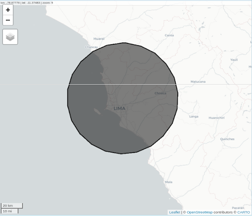
vector <- ee$Geometry$Point(-77.011,-11.98) %>% |
Fig. F6.4.4 A polygon buffer surrounding the city of Lima, Peru |
Next, Earth Engine feature collections (Fig. F6.4.5).
building <- ee$FeatureCollection$Dataset$ |
Fig. F6.4.5 Building footprints in Lagos, Nigeria |

The rgee functionality also supports the display of ee$ImageCollection via Map$addLayers (note the extra “s” at the end). Map$addLayers will use the same visualization parameters for all the images (Fig. F6.4.6). If you need different visualization parameters per image, use a Map$addLayer within a for loop.
# Define a ImageCollection |
Fig. F6.4.6 MOD16A2 total evapotranspiration values (kg/m^2/8day) |

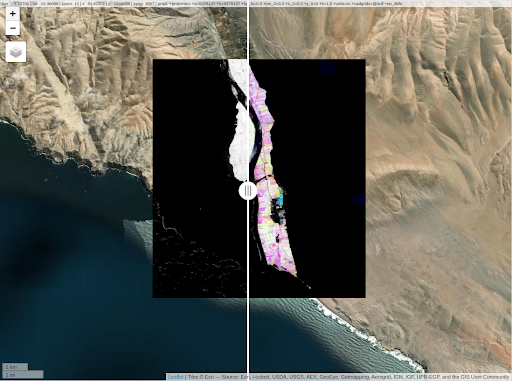
Another useful rgee feature is the comparison operator (|), which creates a slider in the middle of the canvas, permitting quick comparison of two maps. For instance, load a Landsat 4 image:
landsat <- ee$Image('LANDSAT/LT04/C01/T1/LT04_008067_19890917') |
Calculate the Normalized Difference Snow Index.
ndsi <- landsat$normalizedDifference(c('B3', 'B5')) |
Define a constant value and use ee$Image$gte to return a binary image where pixels greater than or equal to that value are set as 1 and the rest are set as 0. Next, filter 0 values using ee$Image$updateMask.
ndsiMasked <- ndsi$updateMask(ndsi$gte(0.4)) |
Define the visualization parameters.
vizParams <- list( |
Center the map on the Huayhuash mountain range in Peru.
Map$setCenter(lon=-77.20, lat=-9.85, zoom=10) |
Finally, visualize both maps using the | operator (Fig. F6.4.7).
m2 <- Map$addLayer(ndsiMasked, ndsiViz, 'NDSI masked') |
Fig. F6.4.7 False-color composite over the Huayhuash mountain range, Peru |

Code Checkpoint F64d. The book’s repository contains information about what your code should look like at this point.
Section 4. Integrating rgee with Other Python Packages
As noted in Sect. 1, rgee set up a Python environment with NumPy and earthengine-api in your system. However, there is no need to limit it to just two Python packages. In this section, you will learn how to use the Python package ndvi2gif to perform a Normalized Difference Vegetation Index (NDVI) multi-seasonal analysis in the Ocoña Valley without leaving R.
Whenever you want to install a Python package, you must run the following.
library(rgee) |
The ee_Initialize function not only authenticates your Earth Engine account but also helps reticulate to set up a Python environment compatible with rgee. After running ee_Initialize, use reticulate::install_python to install the desired Python package.
py_install("ndvi2gif") |
The previous procedure is needed just once for each Python environment. Once installed, we simply load the package using reticulate::import.
ngif <- import("ndvi2gif") |
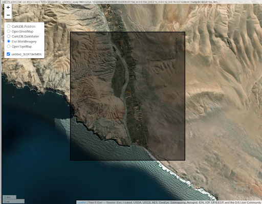
Then, we define our study area using ee$Geometry$Rectangle (Fig. F6.4.8), and use the leaflet layers control to switch between basemaps.
colca <- c(-73.15315, -16.46289, -73.07465, -16.37857) |
Fig. F6.4.8 A rectangle drawn over the Ocoña Valley, Peru |
In ndvi2gif, there is just one class: NdviSeasonality. It has the following four public methods.
- get_export: Exports NDVI year composites in .GeoTIFF format to your local folder.
- get_export_single: Exports single composite as .GeoTIFF to your local folder.
- get_year_composite: Returns the NDVI composites for each year.
- get_gif: Exports NDVI year composites as a .gif to your local folder.
To run, the NdviSeasonality constructor needs to define the following arguments.
- roi: the region of interest
- start_year: the initial year to start to create yearly composites
- end_year: the end year to look for
- sat: the satellite sensor
- key: the aggregation rule that will be used to generate the yearly composite
For each year, the get_year_composite method generates an NDVI ee$Image with four bands, one band per season. Color combination between images and bands will allow you to interpret the vegetation phenology over the seasons and years. In ndvi2gif, the seasons are defined as follows.
- winter =c('-01-01', '-03-31')
- spring=c('-04-01', '-06-30')
- summer=c('-07-01', '-09-30')
- autumn=c('-10-01', '-12-31')
myclass <- ngif$NdviSeasonality( |
We can display maps interactively using the Map$addLayer (Fig. F6.4.9), and use the leaflet layers control to switch between basemaps.
Map$addLayer(wintermax, list(min=0.1, max=0.8), 'winterMax') | |
Fig. F6.4.9 Comparison between the maximum historic winter NDVI and the mean historic NDVI. Colors represent the season when the maximum value occurred. |
And we can export the results to a GIF format.
myclass$get_gif() |
To get more information about the ndvi2gif package, visit its GitHub repository.
Code Checkpoint F64e. The book’s repository contains information about what your code should look like at this point.
Section 5. Converting JavaScript Modules to R
In recent years, the Earth Engine community has developed a lot of valuable third-party modules. Some incredible ones are geeSharp (Zuspan 2020), ee-palettes (Donchyts et al. 2020), spectral (Montero 2021), and LandsatLST (Ermida et al. 2020). While some of these modules have been implemented in Python and JavaScript (e.g., geeSharp and spectral), most are available only for JavaScript. This is a critical drawback, because it divides the Earth Engine community by programming languages. For example, if an R user wants to use tagee (Safanelli et al. 2020), the user will have to first translate the entire module to R.
In order to close this breach, the ee_extra Python package has been developed to unify the Earth Engine community. The philosophy behind ee_extra is that all of its extended functions, classes, and methods must be functional for the JavaScript, Julia, R, and Python client libraries. Currently, ee_extra is the base of the rgeeExtra (Aybar et al. 2021) and eemont (Montero 2021) packages.
To demonstrate the potential of ee_extra, let’s study an example from the Landsat Land Surface Temperature (LST) JavaScript module. The Landsat LST module computes the land surface temperature for Landsat products (Ermida et al. 2020). First we will run it in the Earth Engine Code Editor; then we will replicate those results in R.
First, JavaScript. In a new script in the Code Editor, we must require the Landsat LST module.
var LandsatLST=require( |
The Landsat LST module contains a function named collection. This function receives the following parameters.
- The Landsat archive ID
- The starting date of the Landsat collection
- The ending date of the Landsat collection
- The region of interest as geometry
- A Boolean parameter specifying if we want to use the NDVI for computing a dynamic emissivity instead of using the emissivity from ASTER
In the following code block, we are going to define all required parameters.
var geometry=ee.Geometry.Rectangle([-8.91, 40.0, -8.3, 40.4]); |
Now, with all our parameters defined, we can compute the land surface temperature by using the collection method from Landsat LST.
var LandsatColl=LandsatLST.collection(satellite, date_start, |
The result is stored as an ImageCollection in the LandsatColl variable. Now select the first element of the collection as an example by using the first method.
var exImage=LandsatColl.first(); |
This example image is now stored in a variable named 'exImage'. Let’s display the LST result on the Map. For visualization purposes, we’ll define a color palette.
var cmap=['blue', 'cyan', 'green', 'yellow', 'red']; |
Then, we’ll center the map in the region of interest.
Map.centerObject(geometry); |
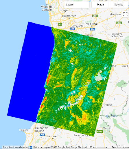
Finally, let’s display the LST with the cmap color palette by using the Map.addLayer method (Fig. F6.4.10). This method receives the image to visualize, the visualization parameters, the color palette, and the name of the layer to show in the layer control. The visualization parameters will be:
- min: 290 (a minimum LST value of 290 K)
- max: 320 (a maximum LST value of 320 K)
- palette: cmap (the color palette that was created some steps before)
The name of the layer in the Map layer set will be LST.
Map.addLayer(exImage.select('LST'),{ |
Fig. F6.4.10 A map illustrating LST, obtained by following the JavaScript example |
Code Checkpoint F64f. The book’s repository contains a script that shows what your code should look like at this point.
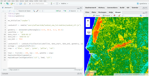
Now, let’s use R to implement the same logic. As in the previous sections, import the R packages: rgee and rgeeExtra. Then, initialize your Earth Engine session.
library(rgee) |
Install rgeeExtra Python dependencies.
py_install(packages=c("regex", "ee_extra", "jsbeautifier")) |
Using the function rgeeExtra::module loads the JavaScript module.
LandsatLST <- module("users/sofiaermida/landsat_smw_lst:modules/Landsat_LST.js") |
The rest of the code is exactly the same as in JavaScript.
geometry <- ee$Geometry$Rectangle(c(-8.91, 40.0, -8.3, 40.4)) |
Fig. F6.4.11 A map illustrating LST, obtained by following the R example |
Code Checkpoint F64g. The book’s repository contains information about what your code should look like at this point.
Question 1. When and why might users prefer to use R instead of Python to connect to Earth Engine?
Question 2. What are the advantages and disadvantages of using rgee instead of the Earth Engine JavaScript Code Editor?
Synthesis
Assignment 1. Estimate the Gaussian curvature map from a digital elevation model using rgee and rgeeExtra. Hint: Use the module 'users/joselucassafanelli/TAGEE:TAGEE-functions'.
Conclusion
In this chapter, you learned how to use Earth Engine and R in the same workflow. Since rgee uses reticulate, rgee also permits integration with third-party Earth Engine Python packages. You also learned how to use Map$addLayer, which works similarly to the Earth Engine User Interface API (Code Editor). Finally, we also introduced rgeeExtra, a new R package that extends the Earth Engine API and supports JavaScript module execution.
Feedback
To review this chapter and make suggestions or note any problems, please go now to bit.ly/EEFA-review. You can find summary statistics from past reviews at bit.ly/EEFA-reviews-stats.
References
Cloud-Based Remote Sensing with Google Earth Engine. (n.d.). CLOUD-BASED REMOTE SENSING WITH GOOGLE EARTH ENGINE. https://www.eefabook.org/
Cloud-Based Remote Sensing with Google Earth Engine. (2024). In Springer eBooks. https://doi.org/10.1007/978-3-031-26588-4
Aybar C, Wu Q, Bautista L, et al (2020) rgee: An R package for interacting with Google Earth Engine. J Open Source Softw 5:2272. https://doi.org/10.21105/joss.02272
Ermida SL, Soares P, Mantas V, et al (2020) Google Earth Engine open-source code for land surface temperature estimation from the Landsat series. Remote Sens 12:1471. https://doi.org/10.3390/RS12091471
Grolemund G (2014) Hands-On Programming with R - Write Your Own Functions and Simulations. O’Reilly Media, Inc.
Lovelace R, Nowosad J, Muenchow J (2019) Geocomputation with R. Chapman and Hall/CRC
Montero D (2021) eemont: A Python package that extends Google Earth Engine. J Open Source Softw 6:3168. https://doi.org/10.21105/joss.03168
Pebesma E, Bivand R (2019) Spatial Data Science. https://r-spatial.org/book/