Cloud-Based Remote Sensing with Google Earth Engine

Fundamentals and Applications

Part A3: Terrestrial Applications

Earth’s terrestrial surface is analyzed regularly by satellites, in search of both change and stability. These are of great interest to a wide cross-section of Earth Engine users, and projects across large areas illustrate both the challenges and opportunities for life on Earth. Chapters in this Part illustrate the use of Earth Engine for disturbance, understanding long-term changes of rangelands, and creating optimum study sites.

Chapter A3.5: Deforestation Viewed from Multiple Sensors

Authors

Xiaojing Tang

Overview

Combining data from multiple sensors is the best way to increase data density and hence detect change faster. The purpose of this chapter is to demonstrate a simple method of combining Landsat, Sentinel-2, and Sentinel-1 data for monitoring tropical forest disturbance. You will learn how to import, preprocess, and fuse optical and synthetic aperture radar (SAR) remote sensing data. You will also learn how to monitor change using time-series models.

Learning Outcomes

• Combining optical and SAR images for change detection.
• Fitting a time-series model to an ImageCollection.
• Using established time-series models to detect anomalies in new images.
• Performing change detection with a rolling monitoring window.
• Monitoring forest disturbance in near real time.

Helps if you know how to:

• Understand the characteristics and preprocessing of Landsat and Sentinel images (Part F1).
• Understand regressions in Earth Engine (Chap. F3.0).
• Work with array images (Chap. F3.1, Chap. F4.6).
• Understand the concept of spectral unmixing (Chap. F3.2).

• Write a function and map it over an ImageCollection (Chap. F4.0).

• Fit linear and nonlinear functions with regression in an ImageCollection time series (Chap. F4.6).
• Export and import results as Earth Engine assets (Chap. F5.0).

Github Code link for all tutorials

This code base is collection of codes that are freely available from different authors for google earth engine.

Github Source

Introduction to Theory 

Deforestation and forest degradation are large sources of carbon emissions and negatively impact biodiversity, food security, and human well-being. The ability to quickly and accurately detect forest disturbance events is essential for preventing future forest loss and mitigating the negative effects. Combining optical and radar data has the potential to achieve faster detection of forest disturbance than using an individual system. The main challenge is the methodological approach for fusing the different datasets. The Fusion Near Real-Time (FNRT) algorithm (Tang et al. 2022) is a monitoring algorithm for tropical forest disturbance that combines data from Landsat, Sentinel-2, and Sentinel-1. For each sensor system, the FNRT algorithm fits time-series models over data from a three-year training period prior to the one-year monitoring period. FNRT then produces a change score for each new observation collected during the monitoring period based on the residuals and the root-mean-square error (RMSE) of the time-series model. The change scores from all three different sensors are then combined to form one dense time series for change detection. In this chapter, we will learn how to run a simplified version of FNRT to monitor forest disturbance in 2020 for a test area located in the Brazilian Amazon.

Practicum

This lab is designed for advanced users of Earth Engine. We assume that you already know how to import and preprocess large quantities of Landsat, Sentinel-2, and Sentinel-1 data as image collections. The code for importing and preprocessing input data will be provided in the example script, but it will not be discussed in detail in this chapter. To learn more about FNRT, refer to Tang et al. (2022).

Section 1. Understand How FNRT Works

For this lab, we will use a graphical user interface to help us understand conceptually how FNRT combines data from different sensors and detects forest disturbance. Fig. A3.5.1 shows the user interface of the app.

Code Checkpoint A35a. The book’s repository contains information about accessing the app.

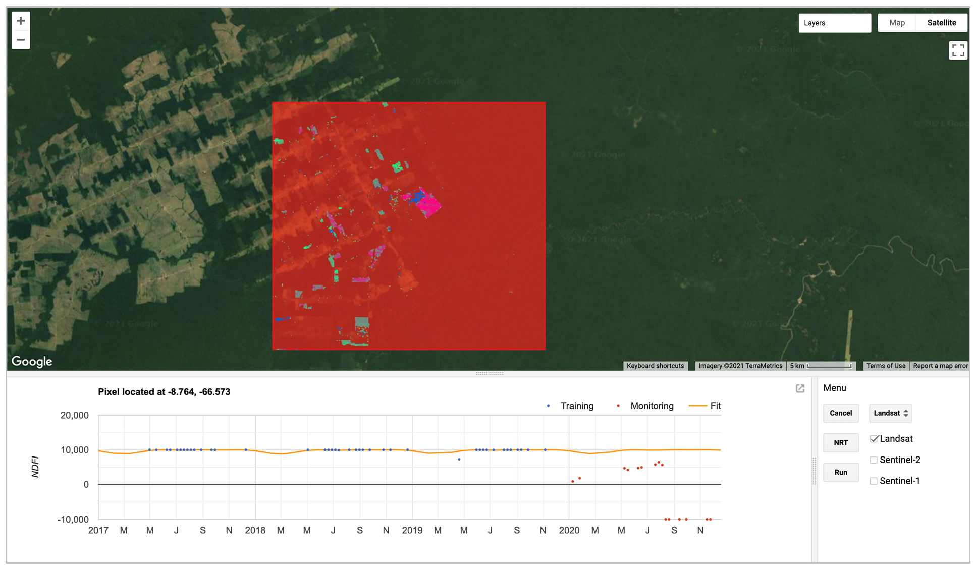
There are three main tools that can be used to explore the FNRT algorithm. Note that only one plotting tool can be activated at a time, and each tool can be deactivated by clicking the button again:

1. The Fit button activates the “fit time-series model” tool, which allows users to click anywhere in the map area, load the time-series data, and fit a harmonic model for the pixel covering the clicked location, using data from the sensor selected in the widget just to the right of the Fit button.
2. The Monitor button activates the “near real-time monitoring” tool, which allows users to click anywhere in the map area and plot the results of FNRT for the pixel covering the clicked location, using data from all the sensors that were checked via the checkbox widgets to the right of the Monitor button.
3. The Run button runs FNRT for the entire test area using data from the sensors that are checked, and loads the resulting forest disturbance map to the map area.

Let’s start by looking at some examples of time series so we have a better understanding of the model. We first need to know where to look for changes. Let’s try to have only “Landsat” checked, and click Run. This will run FNRT with only Landsat data and quickly produce a forest disturbance map for 2020 (Fig. A3.5.2a). Now click Fit to activate the “Fit time-series model” tool, and then click on a pixel that shows forest disturbance activity according to the map. Wait a few seconds to let the app generate the time-series plot in the time series panel. Once it is completed, you should see a plot similar to Fig. A3.5.2c.

The model-fit plot (Fig. A3.5.2c) shows data from Landsat for the training period (blue) and monitoring period (red). It also shows a harmonic time-series model fit to the training data (orange line). The model fit extends into the monitoring period, which represents the model prediction. Notice that the satellite observations (red points) are very close to the model fit before the forest disturbance occurs. After the disturbance, the observations deviate away from the model fit. The algorithm monitors change by keeping track of differences between the observations and the model predictions.

Now click Monitor to activate the “near real-time monitoring” tool, and click the same pixel in the map. The app will then make a plot similar to (d) in Fig. A3.5.2. The near real-time monitoring plot (Fig. A3.5.2d) shows the change scores (Z-score) for the training and the monitoring period. A large change score indicates that something looks different in the satellite image. But sometimes that can be caused by a cloud or a cloud shadow that slipped through the masking process (e.g., the large change scores in the training period). Therefore, the monitoring algorithm looks for multiple large scores within a short monitoring window as an indicator of real forest disturbance.

The monitoring algorithm works through all the observations available during the monitoring period chronologically. Using baseball as an analogy, we flag each change score above a threshold as a “strike” and each change score below the threshold as a “ball.” If the algorithm finds multiple strikes in a short monitoring window, a “strikeout” would then be called on the pixel and the date of the first strike would be recorded as the date of change (Fig. A3.5.2d).

Question 1. How many strikes were detected before a forest disturbance was confirmed (strikeout)?

When performing multi-sensor data fusion, FNRT would fit a separate time-series model and calculate change scores using data from each sensor (Fig. 3.4.3a–c). The change scores calculated using data from the three sensors are then combined, and change monitoring is applied to the combined scores (Fig. 3.4.4d).

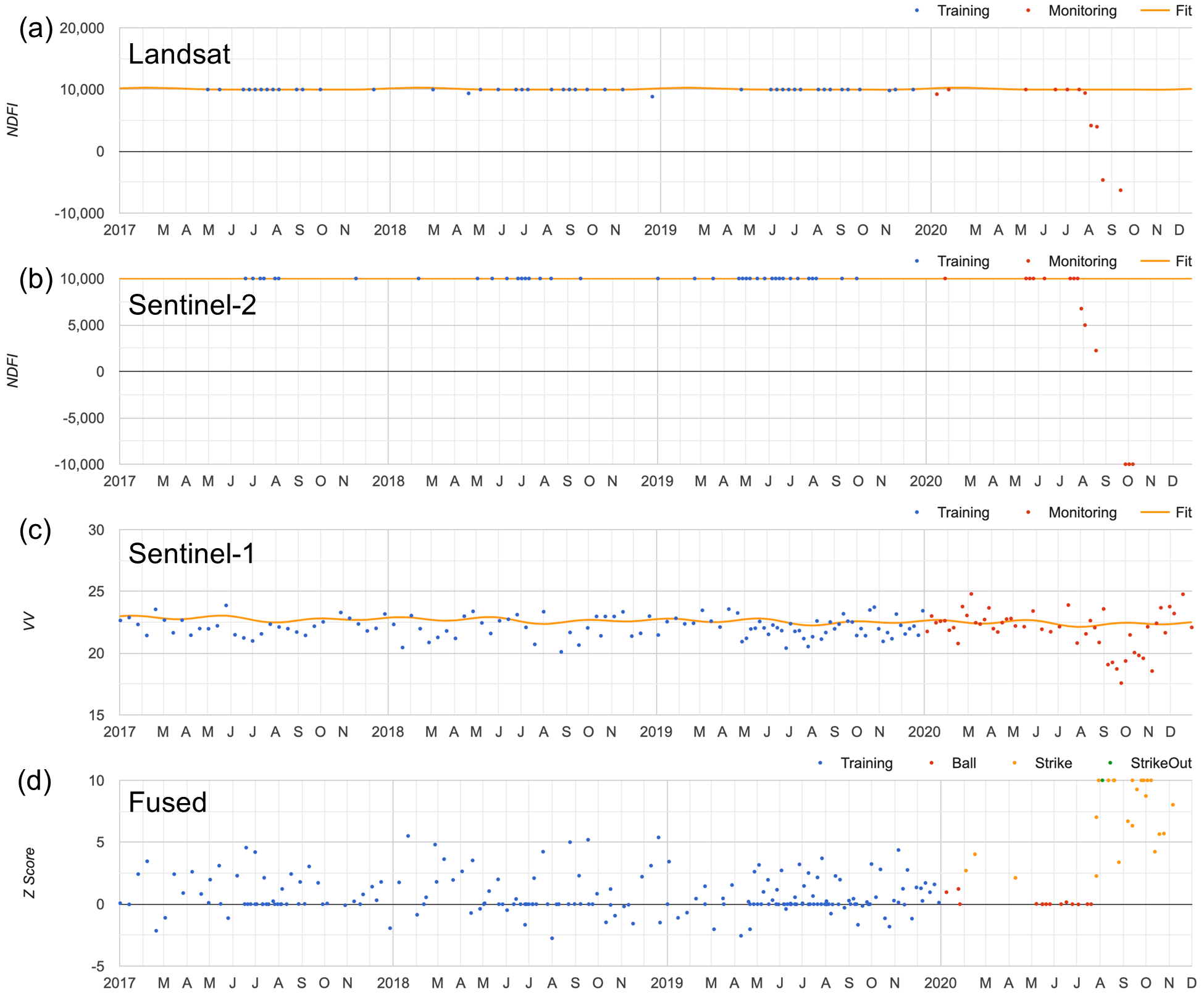
The FNRT app also allows us to run change monitoring for the entire test area by clicking the Run button. A forest disturbance map showing the date of the disturbances is then added to the map. The users can use the checkbox widgets to choose which data stream is included in the process of making the map (e.g., Fig. A3.5.4). In general, optical data is more sensitive to forest disturbance than SAR data. Combining multiple data streams can help detect the disturbance earlier, compared to using data from each individual sensor.

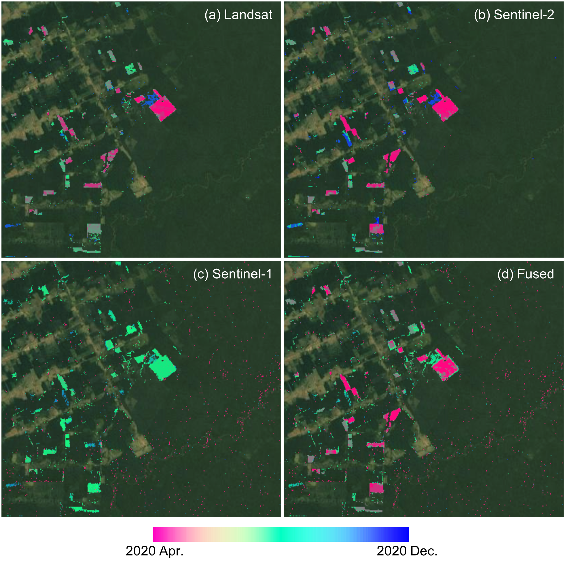
Question 2. Can you find forest disturbances that were detected earlier through the use of data from all three sensors rather than using just Landsat data?

Now that we understand conceptually how FNRT works, let’s create a simple script to implement it.

Section 2. Define Study Area and Model Parameters

Section 2.1. Study Area

There are several ways to define a study area: 1) import an existing FeatureCollection from an Earth Engine asset; 2) use the drawing tool of the Code Editor; and 3) create a polygon by entering the coordinates. Here we select a box, approximately 20 km by 20 km, located in the Brazilian Amazon as our study area.

Note that because of the complexity of the FNRT algorithm, it requires quite a lot of computational resources and can result in a “User Memory Limit” error if applied to too large of an area. Divide the study area into multiple tiles if you are trying to monitor a large area.

Section 2.2. Model Parameters

A few model parameters need to be defined and can be tuned to optimize the algorithm for specific regions or monitoring conditions.

For demonstration of the algorithm, we define the year 2020 as our monitoring period (monitorPeriod). We then recommend using the three years prior to the monitoring period as the training period (trainPeriod) to establish baseline time-series models.

A few parameters can be used to control the sensitivity of the algorithm: a z-threshold (z) defines the minimum change score required to flag a possible change observation; an m-size (m) defines the size of the monitoring window, or how many consecutive observations we check for change; and an n-change (n) defines the number of possible change observations within the monitoring window required to confirm a forest disturbance.

For each sensor we also need to select the band (band) to use for monitoring; a minimum RMSE (minRMSE) to prevent overly sensitive detection caused by unusually good model fit; and a strike-only flag (strikeOnly) to allow a data stream to contribute only to confirmation of a change.

Code Checkpoint A35b. The book’s repository contains a script that shows what your code should look like at this point.

Section 3. Import and Preprocess Data

We need to import data from each sensor for the training period and the monitoring period as two seperate image collections. Each image in the ImageCollection needs to be preprocessed. For optical data, we need to apply spectral unmixing and calculate the Normalized Difference Fraction Index (NDFI) (Souza et al. 2005). Since spectral unmixing would be applied to both Landsat and Sentinel-2 data, let’s first implement a common “unmixing” function.

Several studies (e.g., Bullock et al. 2020, Chen et al. 2021) have shown that spectral unmixing and NDFI work very well in detecting tropical forest disturbance. Here we use the same endmembers used in Souza et al. (2005) for the spectral unmixing, and calculate NDFI based on Equations 4 and 5 in Souza et al. (2005).

For Landsat data, we need to load the Landsat 7 and Landsat 8 Surface Reflectance product as an ImageCollection. We can filter the collection based on our study area and time period. Each image in the ImageCollection is masked based on the QA band; then spectral unmixing is applied and NDFI calculated. The loadLandsatData function is provided for importing and preprocessing Landsat data.

Preprocessing of Sentinel-2 data is similar to that of Landsat data because they are both optical remote sensing data and are almost identical in many ways. We need to load the Sentinel-2 top-of-atmosphere product (surface reflectance data do not have long enough time series for our purpose) and the Sentinel-2 cloud probability product as image collections, and filter based on our study area and time period. We then join the two collections. Each image in the collection is then masked based on both the QA band and the cloud probability.

For Sentinel-1 data, we use the Sentinel-1 SAR GRD product. Preprocessing of Sentinel-1 data includes: 1) calculation of backscattering; 2) calculation of the ratio of VH and VV; 3) calculation of three-pixel spatial mean; 4) choice of the orbital pass with the most data for the region of interest; and 5) radiometric slope correction using volume model. Please refer to Mullissa et al. (2021) for more detail on the preprocessing of SAR data.

Here we assume you have already learned how to load and preprocess large quantities of Landsat, Sentinel-2, and Sentinel-1 data. We will not discuss these steps in detail here in this lab. Instead, three functions (loadLandsatData, loadS2Data, and loadS1Data) are provided in a separate script with which we can import using the require function. Now we can load all the required input data. We also need to apply the spectral unmixing and calculate NDFI for the Landsat and Sentinel-2 data.

In addition to the remote sensing data, we also need to create a forest mask to limit our monitoring to forested areas. Here we will use the Hansen Global Forest Change dataset. We first use the “tree canopy cover” layer to find areas that had larger than 50% canopy cover in 2000. We then remove all the forest loss area during 2001–2019 and add in all the forest gain from 2000–2012 to create a mask of forested area by the beginning of our monitoring period.

Before we move on to the next section, let’s do some simple checking. Print out the image collections and check whether the correct data is loaded. You can also load the forest mask and visually examine the quality of the mask.

Question 3. How many images are available from each sensor for our monitoring period? Are you surprised by the numbers? (Note that one sensor may have more data because the study area happened to be in the side-lap zone where two orbit passes overlap.) What bands are included in the data of each sensor?

Code Checkpoint A35c. The book’s repository contains a script that shows what your code should look like at this point.

Section 4. Establish Baseline Time Series Model

Before we can monitor change in near real time, we need to establish baseline time-series models using the data of the training period, so that we know what to expect from new observations in the monitoring period. Due to the different physical nature of optical and radar data, it is easier to fit a separate time-series model to data from each sensor. Here we use a harmonic time-series model similar to the one used in the Continuous Change Detection and Classification (CCDC) algorithm (Zhu and Woodcock 2014). Because the timestamps of all the input images are stored in the unit of milliseconds while the harmonic model prefers a unit of years, we first need to define a function to convert any date object into the unit of fractional year (e.g. 2015-03-01 to 2015.1612).

Here we define a function (fitHarmonicMode) to fit a harmonic model to an ImageCollection of time-series data. We first construct the dependent variables according to Equation 1 in Zhu and Woodcock (2014) and add them to each of the input images as new bands (using addDependents function). Then we use a reducer (ee.Reducer.robustLinearRegression) to fit the model to the data using robust linear regression. The function returns the model coefficients and the model RMSE.

With this function (fitHarmonicModel) we can fit the harmonic time-series model to the training data of all three sensors. It is always a good practice to also add some metadata to the results for future reference. The model fitting process will take a few minutes and quite a lot of computer memory. Therefore it is recommended that we run them as tasks and save the results as assets before we proceed to the next step.

Run the script. The model fitting results in export tasks to create assets. Instead of exporting the results for this exercise, however, you should proceed to the next section. In that section we will continue with a precomputed asset that is the same as what the above tasks would create.

Code Checkpoint A35d. The book’s repository contains a script that shows what your code should look like at this point.

Section 5. Create Predicted Values for the Monitoring Period

We will now start exploring the pre-exported results mentioned in the previous section. Place this code below the checkpoint of the previous section:

In this section we will use the time-series models that we produced in Section 4 to create a predicted image (also commonly referred to as a synthetic image; see Zhu et al. 2015) for any given date. The predicted image can give us a good estimate of the reflectance (or index such as NDFI) value of a place assuming no change has occurred. We can then compare the predicted image to the image collected by the satellite on the same date. Areas that look very different would likely be areas that have changed. Note that all the coefficients of the harmonic model were saved as a single-band array. So the very first step here is to define a function dearrayModel to convert the array image into a multiband image with each coefficient in one band.

Second, we need to define a function that creates a predicted image for all the dates for which a real image is available during the monitoring period.

The createPredImg function calculates a predicted image based on the date of the real image and the model coefficients. It returns a new image with both the predicted image and the real image.

We can then apply the createPredImg function to each image in the image collections of the monitoring data. We can define another function to map over an ImageCollection to apply createPredImg to all images in the collection.

Let’s apply addPredicted to monitoring data of all three sensors. Note this process is still sensor-specific. Let’s print out the result for Landsat to examine the structure of the output.

Question 4. How many images are in the ImageCollection of the predicted images? Is it the same number as the original ImageCollection of the monitoring data? 

Code Checkpoint A35e. The book’s repository contains a script that shows what your code should look like at this point.

Section 6. Calculate Change Scores

Assuming a good model fit, the predicted image would be very close to the real image of the same date for areas with no change. So what we need to do now is examine each pair of real and predicted images and look for areas where they differ from each other. And if we merge the three data streams, we would be able to significantly increase the data density and potentially detect changes faster. But before we can fuse the three data streams together, we need to produce a normalized measurement of the likelihood of change.

The FNRT algorithm calculates a change score (Tang et al. 2019) very similar to a z-score. First, it calculates the residuals defined as the difference between the predicted value and the observed value. The residuals are then scaled with the RMSE of the time-series model to get the change score. If a change score is above the preset threshold (z in the parameters), then it is flagged as “possible change” (or a “strike” in baseball terminology). The implementation of this part is quite simple:  

Note that here we restrict the predicted value to be under 10000 because that is the theoretical maximum for NDFI.

We also need to have a minimum RMSE (minRMSE) when scaling the residuals. This is because when using indices such as NDFI, it is sometimes possible to have perfect model fits resulting in very low or even zero RMSE, which would then cause the model to be overly sensitive to subtle variations in the monitoring data. The minRMSE is calculated for each pixel as a percentage of the average values of all observations in the training period.

For this particular implementation of FNRT, the determination of a strike is directional, meaning that we are looking for changes only in one direction. This is because we already expect that a forest disturbance will cause a decrease in NDFI or VV backscattering. Modification would be required if monitoring in another direction (e.g., if using SWIR reflectance) or bidirectional monitoring is desired. Let’s apply the two new functions to our three data streams:

Code Checkpoint A35f. The book’s repository contains a script that shows what your code should look like at this point.

Question 5. What bands are included in the change scores images?

Section 7. Multisensor Data Fusion and Change Detection

Now we are finally ready to fuse the three data streams together. This step is quite straightforward: we just need to merge the three image collections of the change scores, and then sort them by their timestamps.

The change monitoring function uses a binary array to keep track of the number of strikes within a monitoring window. The size of the monitoring window is defined by the model parameters (nrtParam.m). The default monitoring window size is five.

We first initiate the monitoring window with a binary array of 0 with a size of five bits (00000) for each pixel. When we iterate through all the change score images chronologically, we shift the binary array left for those pixels that were not masked in the current change score image (00000 → 0000). We then append the current change flag (strike or not) to the shifted binary array (0000 → 00001). The process continues, as we iterate through all the change scores images (e.g., 00001 → 00011 → 00110 → 01101 → 11011). Every time a new value is appended to the binary array, we also check how many strikes (1s) are there. If the number of strikes exceeds the required number (nrtParam.n) to flag a change, then a change is flagged and the date of the change recorded.

Now we apply the monitoring function (monitorChange) to the fused data (fused) using the default model parameters (nrtParam). We can then add the result, the forest disturbance map, to the map panel to visually examine it.

Code Checkpoint A35g. The book’s repository contains a script that shows what your code should look like at this point.

If we run the whole script now, we can create a map of forest disturbance that occurred in 2020 for our test area. The visualization of the map shows us the timing of all the forest disturbance detected by the FNRT algorithm (Fig. A3.5.5). You will notice a few large disturbance events. There may also be some tiny speckles, which are likely errors of commission. Try adjusting the monitoring parameters (nrtParam) to see if you can improve the map. Another common practice is to apply a spatial filter to filter out scattered single pixels of change (Bullock et al. 2020).

Question 6. Can you run the change detection without Sentinel-1 input or with just Landsat input? Was forest disturbance detected faster when we used data from all three sensors?

Synthesis

Now that you have learned how to implement the simplified version of FNRT for the test area that we selected, let’s try to use it to do some real monitoring of tropical forest disturbance.

Assignment 1. Modify the code and apply it in a different area of your choice. Note that you will need to keep the area small in order to be able to run everything easily in the Code Editor.

Assignment 2.  Try to monitor more recent changes by changing the monitoring period to 2021. Note you would need to change the training period to 2018–2020, and also update the forest mask.

Assignment 3. If you want to try a more challenging task, you can integrate your results into the FNRT app that we used in Sect. 1.

Conclusion

In this chapter we experimented with a simple way to combine data from three different sensors (Landsat, Sentinel-2, and Sentinel-1) for the purpose of detecting tropical forest disturbance as early as possible. We started with loading and preprocessing the input data. We learned how to fit a harmonic model to time-series data, and how to make predicted observations based on a model fit. We also learned how to look for changes with a moving monitoring window over a time series of change scores. The full FNRT algorithm is more complex than the “lite” version that we implemented in this lab. If interested, please refer to Tang et al. (2022) for more details.

Feedback

To review this chapter and make suggestions or note any problems, please go now to bit.ly/EEFA-review. You can find summary statistics from past reviews at bit.ly/EEFA-reviews-stats.

References

Cloud-Based Remote Sensing with Google Earth Engine. (n.d.). CLOUD-BASED REMOTE SENSING WITH GOOGLE EARTH ENGINE. https://www.eefabook.org/

Cloud-Based Remote Sensing with Google Earth Engine. (2024). In Springer eBooks. https://doi.org/10.1007/978-3-031-26588-4

Bullock EL, Woodcock CE, Olofsson P (2020) Monitoring tropical forest degradation using spectral unmixing and Landsat time series analysis. Remote Sens Environ 238:110968. https://doi.org/10.1016/j.rse.2018.11.011

Chen S, Woodcock CE, Bullock EL, et al (2021) Monitoring temperate forest degradation on Google Earth Engine using Landsat time series analysis. Remote Sens Environ 265:112648. https://doi.org/10.1016/j.rse.2021.112648

Mullissa A, Vollrath A, Odongo-Braun C, et al (2021) Sentinel-1 SAR backscatter analysis ready data preparation in Google Earth Engine. Remote Sens 13:1954. https://doi.org/10.3390/rs13101954

Souza Jr CM, Roberts DA, Cochrane MA (2005) Combining spectral and spatial information to map canopy damage from selective logging and forest fires. Remote Sens Environ 98:329–343. https://doi.org/10.1016/j.rse.2005.07.013

Tang X, Bratley KE, Cho K, et al (2022) Near real-time monitoring of tropical forest disturbance by fusion of Landsat, Sentinel-2, and Sentinel-1 data. Remote Sens Environ, in review 

Tang X, Bullock EL, Olofsson P, et al (2019) Near real-time monitoring of tropical forest disturbance: New algorithms and assessment framework. Remote Sens Environ 224:202–218. https://doi.org/10.1016/j.rse.2019.02.003

Zhu Z, Woodcock CE (2014) Continuous change detection and classification of land cover using all available Landsat data. Remote Sens Environ 144:152–171. https://doi.org/10.1016/j.rse.2014.01.011

Zhu Z, Woodcock CE, Holden C, Yang Z (2015) Generating synthetic Landsat images based on all available Landsat data: Predicting Landsat surface reflectance at any given time. Remote Sens Environ 162:67–83. https://doi.org/10.1016/j.rse.2015.02.009