Cloud-Based Remote Sensing with Google Earth Engine

Fundamentals and Applications

Part F1: Programming and Remote Sensing Basics

In order to use Earth Engine well, you will need to develop basic skills in remote sensing and programming. The language of this book is JavaScript, and you will begin by learning how to manipulate variables using it. With that base, you’ll learn about viewing individual satellite images, viewing collections of images in Earth Engine, and how common remote sensing terms are referenced and used in Earth Engine.

Chapter F1.3: The Remote Sensing Vocabulary

Authors

Karen Dyson, Andréa Puzzi Nicolau, David Saah, Nicholas Clinton

Overview

The purpose of this chapter is to introduce some of the principal characteristics of remotely sensed images and how they can be examined in Earth Engine. We discuss spatial resolution, temporal resolution, and spectral resolution, along with how to access important image metadata. You will be introduced to image data from several sensors aboard various satellite platforms. At the completion of the chapter, you will be able to understand the difference between remotely sensed datasets based on these characteristics, and how to choose an appropriate dataset for your analysis based on these concepts.  

Learning Outcomes

• Understanding spatial, temporal, and spectral resolution.
• Navigating the Earth Engine Console to gather information about a digital image, including resolution and other data documentation.

Assumes you know how to:

• Navigate among Earth Engine result tabs (Chap. F1.0).
• Visualize images with a variety of false-color band combinations (Chap. F1.1).

Introduction to Theory

Images and image collections form the basis of many remote sensing analyses in Earth Engine. There are many different types of satellite imagery available to use in these analyses, but not every dataset is appropriate for every analysis. To choose the most appropriate dataset for your analysis, you should consider multiple factors. Among these are the resolution of the dataset—including the spatial, temporal, and spectral resolutions—as well as how the dataset was created and its quality.

The resolution of a dataset can influence the granularity of the results, the accuracy of the results, and how long it will take the analysis to run, among other things. For example, spatial resolution, which you will learn more about in Sect. 1, indicates the amount of Earth’s surface area covered by a single pixel. One recent study compared the results of a land use classification (the process by which different areas of the Earth’s surface are classified as forest, urban areas, etc.) and peak total suspended solids (TSS) loads using two datasets with different spatial resolution. One dataset had pixels representing 900 m2 of the Earth’s surface, and the other represented 1 m2. The higher resolution dataset (1 m2) had higher accuracy for the land use classification and better predicted TSS loads for the full study area. On the other hand, the lower resolution dataset was less costly and required less analysis time (Fisher et al. 2018).

Temporal and spectral resolution can also strongly affect analysis outcomes. In the Practicum that follows, we will showcase each of these types of resolution, along with key metadata types. We will also show you how to find more information about the characteristics of a given dataset in Earth Engine.

Github Code link for all tutorials

This code base is collection of codes that are freely available from different authors for google earth engine.

Github Source

Practicum

Section 1. Searching for and Viewing Image Collection Information

If you have not already done so, be sure to add the book’s code repository to the Code Editor by entering https://code.earthengine.google.com/?accept_repo=projects/gee-edu/book into your browser. The book’s scripts will then be available in the script manager panel. If you have trouble finding the repo, you can visit this link for help.

Earth Engine’s search bar can be used to find imagery and to locate important information about datasets in Earth Engine. Let’s use the search bar, located above the Earth Engine code, to find out information about the Landsat 7 Collection 2 Raw Scenes. First, type “landsat 7 collection 2” into the search bar (Fig. F1.3.1). Without hitting Enter, matches to that search term will appear.

Now, click on USGS Landsat 7 Collection 2 Tier 1 Raw Scenes. A new inset window will appear (Fig. F1.3.2).

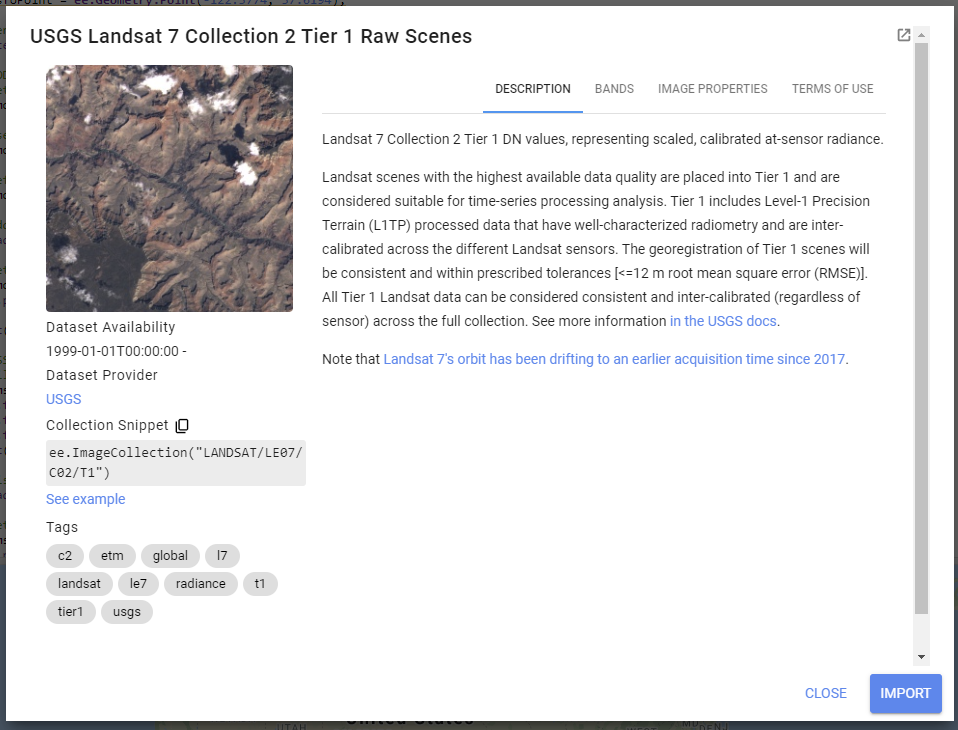
The inset window has information about the dataset, including a description, bands that are available, image properties, and terms of use for the data across the top. Click on each of these tabs and read the information provided. While you may not understand all of the information right now, it will set you up for success in future chapters.

On the left-hand side of this window, you will see a range of dates when the data is available, a link to the dataset provider’s webpage, and a collection snippet. This collection snippet can be used to import the dataset by pasting it into your script, as you did in previous chapters. You can also use the large Import button to import the dataset into your current workspace. In addition, if you click on the See example link, Earth Engine will open a new code window with a snippet of code that shows code using the dataset. Code snippets like this can be very helpful when learning how to use a dataset that is new to you.

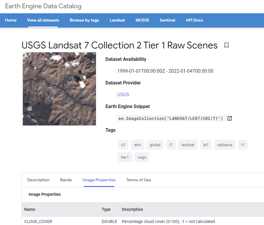
For now, click on the small “pop out” button in the upper right corner of the window. This will open a new window with the same information (Fig. F1.3.3); you can keep this new window open and use it as a reference as you proceed.

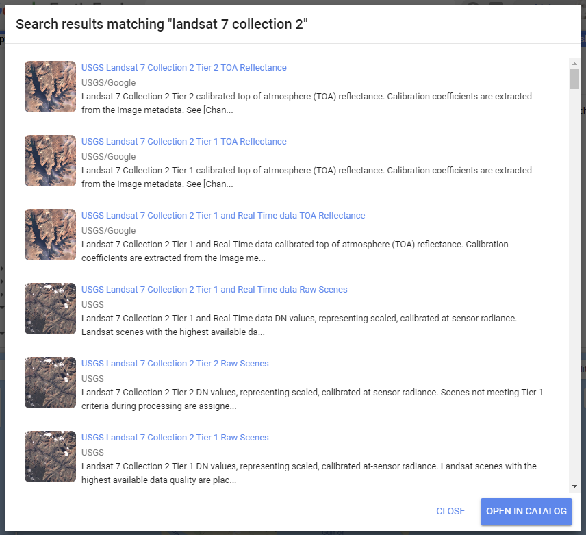
Switch back to your code window. Your “landsat 7 collection 2” search term should still be in the search bar. This time, click the “Enter” key or click on the search magnifying glass icon. This will open a Search results inset window (Fig. F1.3.4).

This more complete search results inset window contains short descriptions about each of the datasets matching your search, to help you choose which dataset you want to use. Click on the Open in Catalog button to view these search results in the Earth Engine Data Catalog (Fig. F1.3.5). Note that you may need to click Enter in the data catalog search bar with your phrase to bring up the results in this new window.

Now that we know how to view this information, let’s dive into some important remote sensing terminology.

Section 2. Spatial Resolution

Spatial resolution relates to the amount of Earth’s surface area covered by a single pixel. It is typically referred to in linear units, for a single side of a square pixel: for example, we typically say that Landsat 7 has “30 m” color imagery. This means that each pixel is 30 m to a side, covering a total area of 900 m2 of the Earth’s surface. Spatial resolution is often interchangeably also referred to as the scale, as will be seen in this chapter when we print that value. The spatial resolution of a given data set greatly affects the appearance of images, and the information in them, when you are viewing them on Earth’s surface.

Next, we will visualize data from multiple sensors that capture data at different spatial resolutions, to compare the effect of different pixel sizes on the information and detail in an image. We’ll be selecting a single image from each ImageCollection to visualize. To view the image, we will draw them each as a color-IR image, a type of false-color image (described in detail in Chap. F1.1) that uses the infrared, red, and green bands. As you move through this portion of the Practicum, zoom in and out to see differences in the pixel size and the image size.

MODIS (on the Aqua and Terra satellites)

As discussed in Chap. F1.2, the common resolution collected by MODIS for the infrared, red, and green bands is 500 m. This means that each pixel is 500 m on a side, with a pixel thus representing 0.25 km2 of area on the Earth’s surface.

Use the following code to center the map on the San Francisco airport at a zoom level of 16.

Let’s use what we learned in the previous section to search for, get information about, and import the MODIS data into our Earth Engine workspace. Start by searching for “MODIS 500” in the Earth Engine search bar.

Use this to import the “MOD09A1.061 Terra Surface Reflectance 8-day Global 500m” ImageCollection. A default name for the import appears at the top of your script; change the name of the import to mod09. 

When exploring a new dataset, you can find the nmes of bands in images from that set by reading the summary documentation, known as the metadata, of the dataset. In this dataset, the three bands for a color-IR image are “sur_refl_b02” (infrared), “sur_refl_b01” (red), and “sur_refl_b04” (green).

In your map window, you should now see something like this.

You might be surprised to see that the pixels, which are typically referred to as “square”, are shown as parallelograms. The shape and orientation of pixels are controlled by the “projection” of the dataset, as well as the projection we are viewing them in. Most users do not have to be very concerned about different projections in Earth Engine, which automatically transfers data between different coordinate systems as it did here. For more details about projections in general and their use in Earth Engine, you can consult the official documentation.

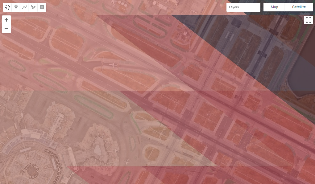
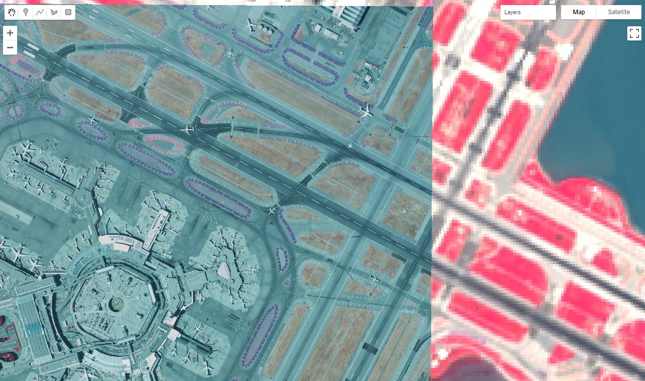
Let’s view the size of pixels with respect to objects on the ground. Turn on the satellite basemap to see high-resolution data for comparison by clicking on Satellite in the upper-right corner of the map window. Then, decrease the layer’s opacity: set the opacity in the Layers manager using the layer’s slider (see Chap. F1.1). The result will look like Fig. F1.3.9.

Print the size of the pixels (in meters) by running this code:

In that call, we used the nominalScale function here after accessing the projection information from the MODIS NIR band. That function extracts the spatial resolution from the projection information, in a format suitable to be printed to the screen. The nominalScale function returns a value just under the stated 500m resolution due to the sinusoidal projection of MODIS data and the distance of the pixel from nadir--that is, where the satellite is pointing directly down at the Earth’s surface.

TM (on early Landsat satellites)

Thematic Mapper (TM) sensors were flown aboard Landsat 4 and 5. TM data have been processed to a spatial resolution of 30m, and were active from 1982 to 2012. Search for “Landsat 5 TM” and import the result called “USGS Landsat 5 TM Collection 2 Tier 1 Raw Scenes”. In the same way you renamed the MODIS collection, rename the import tm. In this dataset, the three bands for a color-IR image are called “B4” (infrared), “B3” (red), and “B2” (green). Let’s now visualize TM data over the airport and compare it with the MODIS data. Note that we can either define the visualization parameters as a variable (as in the previous code snippet) or place them in curly braces in the Map.addLayer function (as in this code snippet).

When you run this code, the TM image will display. Notice how many more pixels are displayed on your screen when compared to the MODIS image.

As we did for the MODIS data, let’s check the scale. The scale is expressed in meters:

MSI (on the Sentinel-2 satellites)

The MultiSpectral Instrument (MSI) flies aboard the Sentinel-2 satellites, which are operated by the European Space Agency. The red, green, blue, and near-infrared bands are captured at 10 m resolution, while other bands are captured at 20 m and 30 m. The Sentinel-2A satellite was launched in 2015 and the 2B satellite was launched in 2017.

Search for “Sentinel 2 MSI” in the search bar, and add the “Sentinel-2 MSI: MultiSpectral Instrument, Level-1C” dataset to your workspace. Name it msi. In this dataset, the three bands for a color-IR image are called “B8” (infrared), “B4” (red), and “B3” (green).

Compare the MSI imagery with the TM and MODIS imagery, using the opacity slider. Notice how much more detail you can see on the airport terminal and surrounding landscape. The 10 m spatial resolution means that each pixel covers approximately 100 m2 of the Earth’s surface, a much smaller area than the TM imagery (900 m2) or the MODIS imagery (0.25 km2).

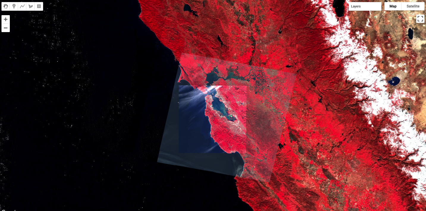
The extent of the MSI image displayed is also smaller than that for the other instruments we have looked at. Zoom out until you can see the entire San Francisco Bay. The MODIS image covers the entire globe, the TM image covers the entire San Francisco Bay and the surrounding area south towards Monterey, while the MSI image captures a much smaller area.

Check the scale of the MSI instrument (in meters):

NAIP

The National Agriculture Imagery Program (NAIP) is a U.S. government program to acquire imagery over the continental United States using airborne sensors. Data is collected for each state approximately every three years. The imagery has a spatial resolution of 0.5–2 m, depending on the state and the date collected.  

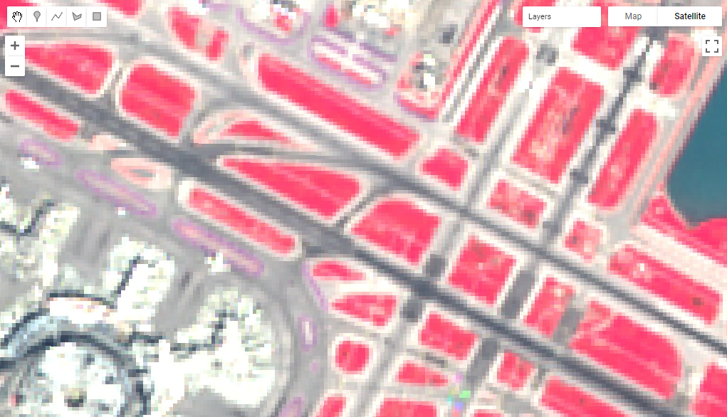
Search for “naip” and import the data set for “NAIP: National Agriculture Imagery Program”.  Name the import naip. In this dataset, the three bands for a color-IR image are called “N” (infrared), “R” (red), and “G” (green).

The NAIP imagery is even more spatially detailed than the Sentinel-2 MSI imagery. However, we can see that our one NAIP image doesn’t totally cover the San Francisco airport. If you like, zoom out to see the boundaries of the NAIP image as we did for the Sentinel-2 MSI imagery.

And get the scale, as we did before.

Each of the datasets we’ve examined has a different spatial resolution. By comparing the different images over the same location in space, you have seen the differences between the large pixels of MODIS, the medium-sized pixels of TM (Landsat 5) and MSI (Sentinel-2), and the small pixels of the NAIP. Datasets with large-sized pixels are also called “coarse resolution,” those with medium-sized pixels are also called “moderate resolution,” and those with small-sized pixels are also called “fine resolution.”

Code Checkpoint F13a. The book’s repository contains a script that shows what your code should look like at this point.

Section 3. Temporal Resolution

Temporal resolution refers to the revisit time, or temporal cadence of a particular sensor’s image stream. Revisit time is the number of days between sequential visits of the satellite to the same location on the Earth’s surface. Think of this as the frequency of pixels in a time series at a given location.

Landsat

The Landsat satellites 5 and later are able to image a given location every 16 days. Let’s use our existing tm dataset from Landsat 5. To see the time series of images at a location, you can filter an ImageCollection to an area and date range of interest and then print it. For example, to see the Landsat 5 images for three months in 1987, run the following code:

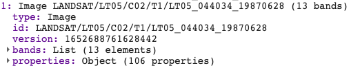
Expand the features property of the printed ImageCollection in the Console output to see a List of all the images in the collection. Observe that the date of each image is part of the filename (e.g., LANDSAT/LT05/C02/T1/LT05_044034_19870628).

However, viewing this list doesn’t make it easy to see the temporal resolution of the dataset. We can use Earth Engine’s plotting functionality to visualize the temporal resolution of different datasets. For each of the different temporal resolutions, we will create a per-pixel chart of the NIR band that we mapped previously. To do this, we will use the ui.Chart.image.series function.

The ui.Chart.image.series function requires you to specify a few things in order to calculate the point to chart for each time step. First, we filter the ImageCollection (you can also do this outside the function and then specify the ImageCollection directly). We select the B4 (near infrared) band and then select three months by using filterDate on the ImageCollection. Next, we need to specify the location to chart; this is the region argument. We’ll use the sfoPoint variable we defined earlier.

By default, this function creates a trend line. It’s difficult to see precisely when each image was collected, so let’s create a specialized chart style that adds points for each observation.

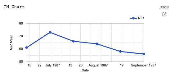
When you print the chart, it will have a point each time an image was collected by the TM instrument (Fig. F1.3.15). In the Console, you can move the mouse over the different points and see more information. Also note that you can expand the chart using the button in the upper right-hand corner. We will see many more examples of charts, particularly in the chapters in Part F4.

Sentinel-2

The Sentinel-2 program’s two satellites are in coordinated orbits, so that each spot on Earth gets visited about every 5 days. Within Earth Engine, images from these two sensors are pooled in the same dataset. Let’s create a chart using the MSI instrument dataset we have already imported.

Compare this Sentinel-2 graph (Fig. F1.3.16) with the Landsat graph you just produced (Fig. F1.3.15). Both cover a period of six months, yet there are many more points through time for the Sentinel-2 satellite, reflecting the greater temporal resolution.

Code Checkpoint F13b. The book’s repository contains a script that shows what your code should look like at this point.

Section 4. Spectral Resolution

Spectral resolution refers to the number and width of spectral bands in which the sensor takes measurements. You can think of the width of spectral bands as the wavelength intervals for each band. A sensor that measures radiance in multiple bands is called a multispectral sensor (generally 3–10 bands), while a sensor with many bands (possibly hundreds) is called a hyperspectral sensor; however, these are relative terms without universally accepted definitions.

Let’s compare the multispectral MODIS instrument with the hyperspectral Hyperion sensor aboard the EO-1 satellite, which is also available in Earth Engine.

MODIS

There is an easy way to check the number of bands in an image:

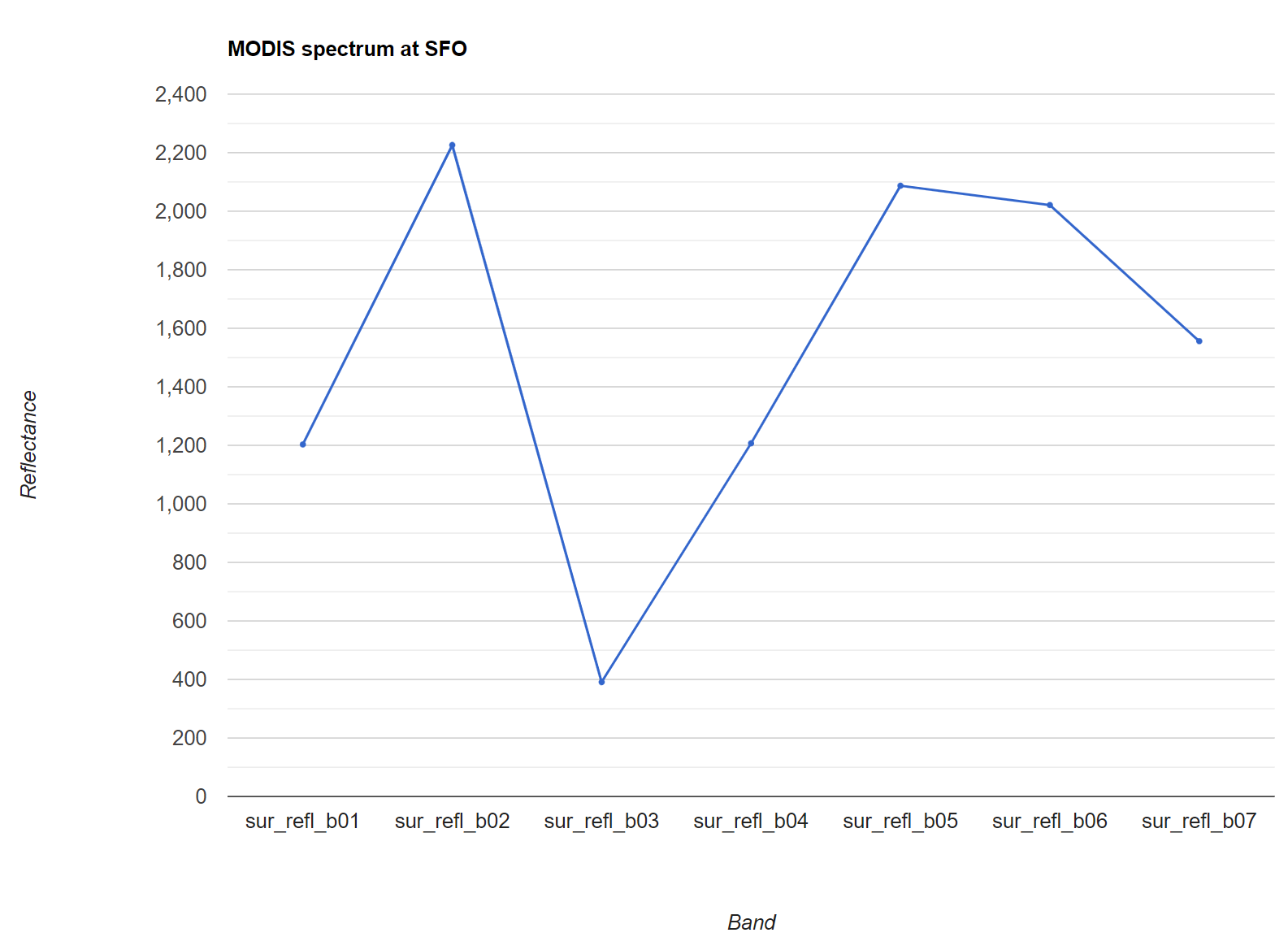
Note that not all of the bands are spectral bands. As we did with the temporal resolution, let’s graph the spectral bands to examine the spectral resolution. If you ever have questions about what the different bands in the band list are, remember that you can find this information by visiting the dataset information page in Earth Engine or the data or satellite’s webpage.

As before, we’ll customize the chart to make it easier to read.

And create a chart using the ui.Chart.image.regions function.

The resulting chart is shown in Fig. F1.3.17. Use the expand button in the upper right to see a larger version of the chart than the one printed to the Console.

EO-1

Now let’s compare MODIS with the EO-1 satellite’s hyperspectral sensor. Search for “eo-1” and import the “EO-1 Hyperion Hyperspectral Imager” dataset. Name it eo1. We can look at the number of bands from the EO-1 sensor.

Examine the list of bands that are printed in the Console. Notice how many more bands the hyperspectral instrument provides.

Now let’s create a reflectance chart as we did with the MODIS data.

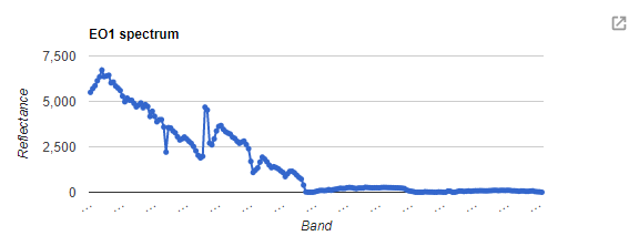
The resulting chart is seen in Fig. F1.3.18. There are so many bands that their names only appear as “...”!

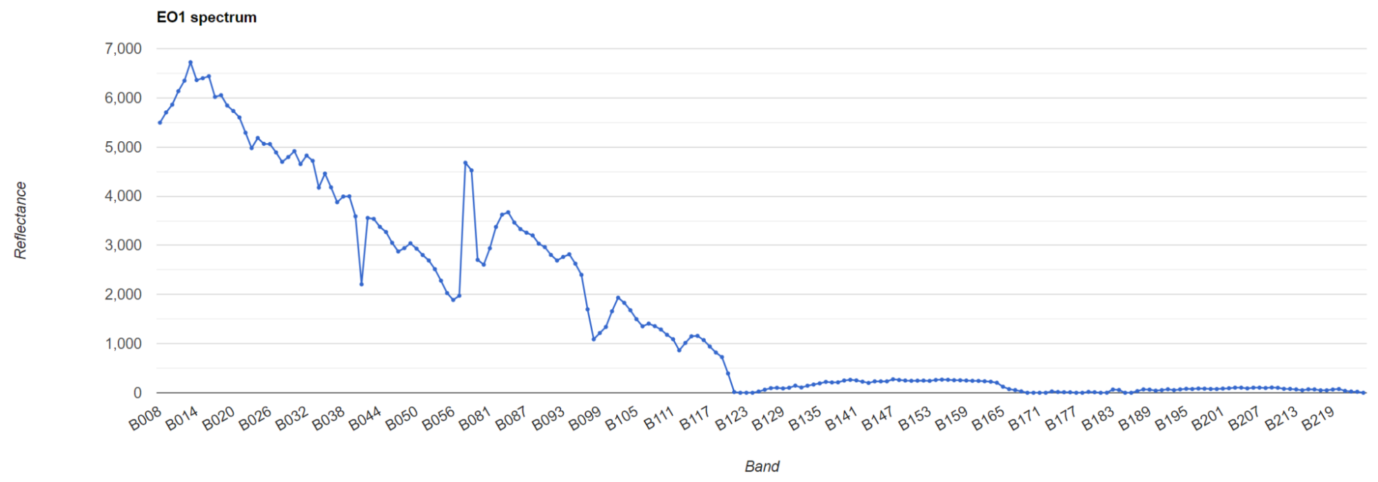
If we click on the expand icon in the top right corner of the chart, it’s a little easier to see the band identifiers, as shown in Fig. F1.3.19. 

Compare this hyperspectral instrument chart with the multispectral chart we plotted above for MODIS.

Code Checkpoint F13c. The book’s repository contains a script that shows what your code should look like at this point.

Section 5. Per-Pixel Quality

As you saw above, an image consists of many bands. Some of these bands contain spectral responses of Earth’s surface, including the NIR, red, and green bands we examined in the Spectral Resolution section. What about the other bands? Some of these other bands contain valuable information, like pixel-by-pixel quality-control data.

For example, Sentinel-2 has a QA60 band, which contains the surface reflectance quality assurance information. Let’s map it to inspect the values.

Use the Inspector tool to examine some of the values. You may see values of 0 (black), 1024 (gray), and 2048 (white). The QA60 band has values of 1024 for opaque clouds, and 2048 for cirrus clouds. Compare the false-color image with the QA60 band to see these values. More information about how to interpret these complex values is given in Chap. F4.3, which explains the treatment of clouds.

Code Checkpoint F13d. The book’s repository contains a script that shows what your code should look like at this point.

Section 6. Metadata

In addition to band imagery and per-pixel quality flags, Earth Engine allows you to access substantial amounts of metadata associated with an image. This can all be easily printed to the Console for a single image.

Let’s examine the metadata for the Sentinel-2 MSI.

Examine the object you’ve created in the Console (Fig. F1.3.20). Expand the image name, then the properties object.

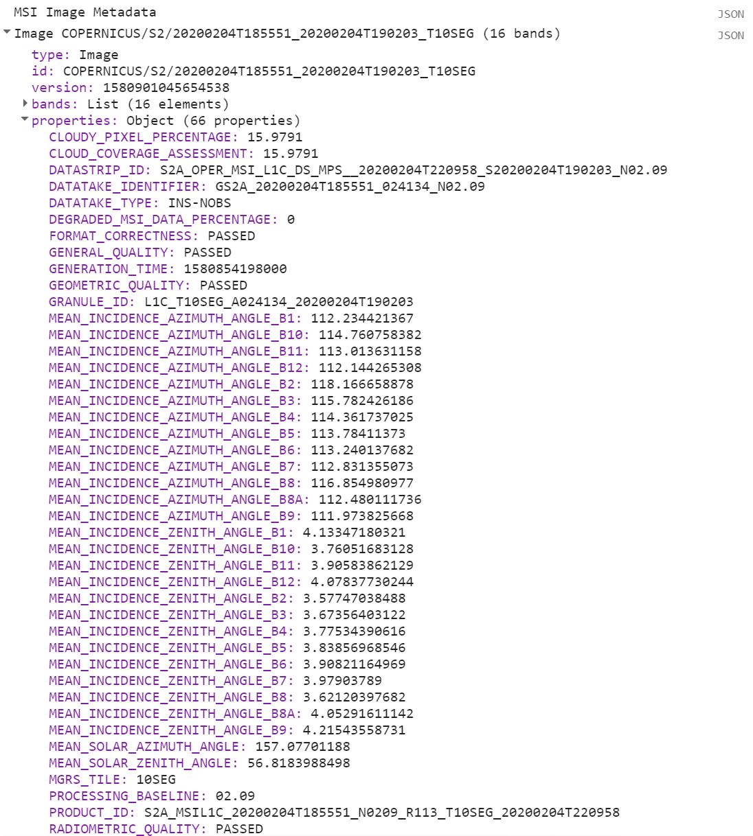
The first entry is the CLOUDY_PIXEL_PERCENTAGE information. Distinct from the cloudiness flag attached to every pixel, this is an image-level summary assessment of the overall cloudiness in the image. In addition to viewing the value, you might find it useful to print it to the screen, for example, or to record a list of cloudiness values in a set of images. Metadata properties can be extracted from an image’s properties using the get function, and printed to the Console.

Code Checkpoint F13e. The book’s repository contains a script that shows what your code should look like at this point.

Synthesis

Assignment 1. Recall the plots of spectral resolution we created for MODIS and EO-1. Create a plot of spectral resolution  for one of the other sensors described in this chapter. What are the bands called? What wavelengths of the electromagnetic spectrum do they correspond to?

Assignment 2. Recall how we extracted the spatial resolution and saved it to a variable. In your code, set the following variables to the scales of the bands shown in Table F1.3.1.

Table F1.3.1         The three datasets and bands to use.

Assignment 3. Make this point in your code: ee.Geometry.Point([-122.30144, 37.80215]). How many MYD09A1 images are there in 2017 at this point? Set a variable called mod09ImageCount with that value, and print it. How many Sentinel-2 MSI surface reflectance images are there in 2017 at this point? Set a variable called msiImageCount with that value, and print it.  

Conclusion

A good understanding of the characteristics of your images is critical to your work in Earth Engine and the chapters going forward. You now know how to observe and query a variety of remote sensing datasets, and can choose among them for your work. For example, if you are interested in change detection, you might require a dataset with spectral resolution including near-infrared imagery and a fine temporal resolution. For analyses at a continental scale, you may prefer data with a coarse spatial scale, while analyses for specific forest stands may benefit from a very fine spatial scale.

Feedback

To review this chapter and make suggestions or note any problems, please go now to bit.ly/EEFA-review. You can find summary statistics from past reviews at bit.ly/EEFA-reviews-stats.

References

Cloud-Based Remote Sensing with Google Earth Engine. (n.d.). CLOUD-BASED REMOTE SENSING WITH GOOGLE EARTH ENGINE. https://www.eefabook.org/

Cloud-Based Remote Sensing with Google Earth Engine. (2024). In Springer eBooks. https://doi.org/10.1007/978-3-031-26588-4

Fisher JRB, Acosta EA, Dennedy-Frank PJ, et al (2018) Impact of satellite imagery spatial resolution on land use classification accuracy and modeled water quality. Remote Sens Ecol Conserv 4:137–149. https://doi.org/10.1002/rse2.61