Cloud-Based Remote Sensing with Google Earth Engine

Fundamentals and Applications

Part A1: Human Applications
This Part covers some of the many Human Applications of Earth Engine. It includes demonstrations of how Earth Engine can be used in agricultural and urban settings, including for sensing the built environment and the effects it has on air composition and temperature. This Part also covers the complex topics of human health, illicit deforestation activity, and humanitarian actions.
Chapter A1.5: Heat Islands
Author
TC Chakraborty
Overview
In this chapter, you will learn about urban heat islands and how they can be calculated from satellite measurements of thermal radiation from the Earth’s surface.
Learning Outcomes
- Understanding how to derive land surface temperature.
- Understanding how to generate urban and rural references.
- Knowing how to calculate the surface urban heat island intensity.
Helps if you know how to:
- Import, filter, and visualize images (Part F1).
- Perform basic image analysis: select bands, compute indices, create masks (Part F2).
- Use expressions to perform calculations on image bands (Chap. F3.1).
- Write a function and map it over an ImageCollection (Chap. F4.0).
- Mask cloud, cloud shadow, snow/ice, and other undesired pixels (Chap. F4.3).
- Conduct basic vector analyses: vectorizing and buffering (Part F5).
- Write a function and map it over a FeatureCollection (Chap. F5.1, Chap. F5.2).
Github Code link for all tutorials
This code base is collection of codes that are freely available from different authors for google earth engine.
Introduction to Theory
Urbanization involves replacement of natural landscapes with built-up structures such as buildings, roads, and parking lots. This land cover modification also changes the properties of the land surface. These changes can range from how much radiation is reflected and absorbed by the surface, to how the heat is dissipated from the surface (for example, removal of vegetation for urban development reduces evaporative cooling). The changes in surface properties can modify local weather and climate (Kalnay and Cai 2003). The most-studied local climate modification due to urbanization is the urban heat island (UHI) effect (Arnfield 2003; Qian et al. 2022). The UHI is the phenomenon in which a city is warmer than either its surroundings or an equivalent surface that is not urbanized. We have known about the UHI effect for almost 200 years (Howard 1833).
Traditionally, the UHI was defined as the difference in air temperature, measured by weather stations, between a city and some rural reference outside the city (Oke 1982). One issue with this method is that different parts of the city can have different air temperatures, making it difficult to capture the UHI for the entire city. Using satellite observations in the thermal bands allows us to get another measure of temperature: the radiometric skin temperature, often known as the land surface temperature (LST). We can use LST to calculate a surface UHI (SUHI) intensity, including how it varies within cities at the pixel scale (Ngie et al. 2014). It is important to stress here that the UHI values observed by satellites and those calculated using air temperature measurements can be very different (Chakraborty et al. 2017, Hu et al. 2019, Venter et al. 2021).
Practicum
Section 1. Deriving Land Surface Temperature
Section 1.1. Deriving Land Surface Temperature from MODIS
Land surface temperature can either be extracted from derived products, such as the MODIS Terra and Aqua satellite products (Wan 2006), or estimated directly from measurements in the thermal band. We will explore both options using the city of New Haven, Connecticut, USA, as the region of interest (Fig. A1.5.1). We will start with the MODIS LST.
We start by loading the feature collection, which, being a census tract-level aggregation, we dissolve to get the overall boundary using the union operation. The FeatureCollection is added to the map for demonstration:
// Load feature collection of New Haven's census tracts from user assets. |

Fig. A1.5.1 Boundary of New Haven, Connecticut
Next we load in the MODIS MYD11A2 version 6 product, which provides eight-day composites of LST from the Aqua satellite. This corresponds to an equatorial crossing time of roughly 1:30 p.m. during daytime and 1:30 a.m. at night. In contrast, the MODIS sensor onboard the Terra platform (MOD11A2 version 6) has an overpass of roughly 10:30 a.m. and 10:30 p.m.
// Load MODIS image collection from the Earth Engine data catalog. |
We want to focus on only summertime SUHI, so we will create a five-year summer composite of LST using a day-of-year filter assembling images from June 1 (day 152) to August 31 (day 243) in each year:
// Create a summer filter. |
We now convert this image into LST in degrees Celsius and mask out all the water pixels (the high specific heat capacity of water would affect LST, and we are focused on land pixels). For the water mask, we use the Global Surface Water dataset (Pekel et al. 2016); to convert the pixel values, we use the scaling factor for the band from the data provider and then subtract by 273.15 to convert from Kelvin to degrees Celsius. The scaling factor can be found in the Earth Engine data summary page (Fig. A1.5.2).
Fig. A1.5.2 Scaling factor in the data summary |

Finally, we clip the image using the city boundary and add the layer to the map.
// Multiply each pixel by scaling factor to get the LST values. |
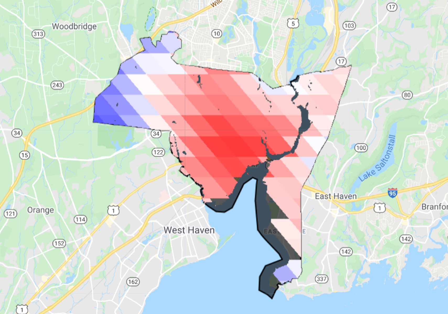
Fig. A1.5.3 Five-year summer composite of daytime MODIS Aqua LST over New Haven, Connecticut. Red pixels show higher LST values and blue pixels have lower values. |
Code Checkpoint A15a. The book’s repository contains a script that shows what your code should look like at this point.
Section 1.2. Deriving Land Surface Temperature from Landsat
Working with MODIS LST is relatively simple because the data are already processed by the NASA team. You can also derive LST from Landsat, which has a much finer native resolution (~30 m) than the ~1 km MODIS pixels. However, you need to derive LST yourself from the measurements in the thermal bands, which also usually involves some estimate of surface emissivity (Li et al. 2013). The surface emissivity (ε) of a material is the effectiveness with which it can emit thermal radiation compared to a black body at the same temperature and can range from 0 (for a perfect reflector) to 1 (for a perfect absorber and emitter). Since the thermal radiation captured by satellites is a function of both LST and ε, you need to accurately prescribe or estimate ε to get to the correct LST. Let’s consider one such simple method using Landsat 8 data.
We will start by loading in the Landsat data, cloud screening and then filtering to a time and region of interest. Continuing in the same script, add the following code:
// Function to filter out cloudy pixels. |
After creating a median composite as a simple way to further reduce the influence of clouds, we mask out the water pixels, and select the brightness temperature band.
// Generate median composite. |
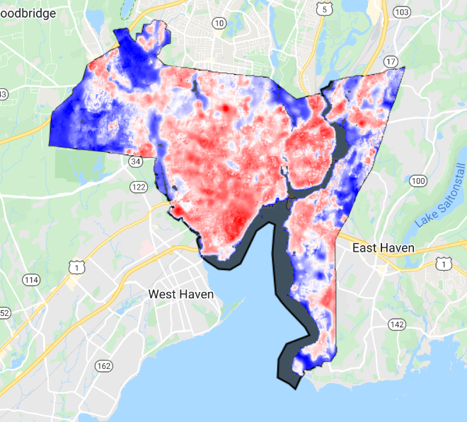
Fig. A1.5.4 Five-year summer median composite of Landsat brightness temperature over New Haven, Connecticut. Red pixels show higher values, and blue pixels have lower values.
Brightness temperature (Fig. A1.5.4) is the temperature equivalent of the infrared radiation escaping the top of the atmosphere, assuming the Earth to be a black body. It is not the same as the LST, which requires accounting for atmospheric absorption and re-emission, as well as the emissivity of the land surface. One way to derive pixel-level emissivity is as a function of the vegetation fraction of the pixel (Malakar et al. 2018). For this, we start by calculating the Normalized Difference Vegetation Index (NDVI) from the Landsat surface reflectance data (see Fig. A1.5.5).
// Calculate Normalized Difference Vegetation Index (NDVI) |

Fig. A1.5.5 Five-year summer median composite of Landsat-derived NDVI over New Haven, Connecticut. White pixels show higher NDVI values, and blue pixels have lower values.
To map NDVI for each pixel to the actual fraction of the pixel with vegetation (fractional vegetation cover), we next use a relationship based on the range of NDVI values for each pixel.
// Find the minimum and maximum of NDVI. Combine the reducers |
Now we use an empirical model of emissivity based on this fractional vegetation cover (Sekertekin and Bonafoni 2020).
// Emissivity calculations. |

Fig. A1.5.6 Surface emissivity over New Haven, Connecticut, based on vegetation fraction. Green pixels show higher values, and white pixels have lower values.
As seen in Fig. A1.5.6, emissivity is lower over the built-up structures compared to over vegetation, which is expected. Note that different models of estimating emissivity would lead to some differences in LST values as well as the SUHI intensity (Sekertekin and Bonafoni 2020, Chakraborty et al. 2021a).
Then we combine this emissivity with the brightness temperature to calculate the LST for each pixel using a simple single-channel algorithm, which is a linearized approximation of the radiation transfer equation (Ermida et al. 2020).
// Calculate LST from emissivity and brightness temperature. |
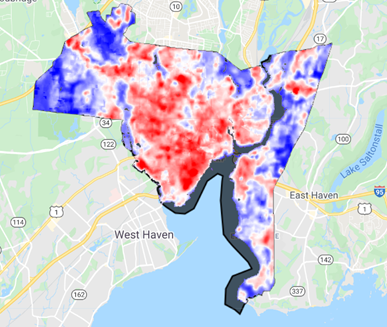
Fig. A1.5.7 Five-year summer median composite of Landsat-derived LST over New Haven, Connecticut. Red pixels show higher LST values, and blue pixels have lower values.
The Landsat-derived values correspond to those of the MODIS Terra daytime overpass. Overall, you do see similar patterns in Figs. A1.5.3 and A1.5.7, but Landsat picks up a lot more heterogeneity than MODIS due to its finer resolution.
Code Checkpoint A15b. The book’s repository contains a script that shows what your code should look like at this point.
Section 1.3. Deriving Land Surface Temperature Using the Earth Engine Landsat LST Toolbox
In the previous section, we explored an LST retrieval algorithm to give an example of the standard steps to get to LST from the satellite measurements in the thermal bands. In this section, we will use an Earth Engine module developed for this purpose to calculate LST (Fig. A1.5.8).
// Link to the module that computes the Landsat LST. |

Fig. A1.5.8 Five-year summer median composite of Landsat-derived LST over New Haven, Connecticut, using the Statistical Mono-Window algorithm. Red pixels show higher LST values, and blue pixels have lower values.
As an aside, the Landsat Collection 2 products have recently incorporated LST bands, which can be processed similar to the MODIS data, but with the bands’ own specific offsets and scaling factors.
Code Checkpoint A15c. The book’s repository contains a script that shows what your code should look like at this point.
Section 2. Defining Urban and Rural References
Now that we have estimates of LST using various products and algorithms, we can calculate the rural LST and subtract from the urban LST to get the SUHI intensity. There are many ways to estimate the rural reference temperature (Li et al. 2022), and we will explore a few of them in this section.
The simplest and probably the most commonly used method to get the rural reference when calculating the SUHI is to generate a buffered area around the urban boundary. The exact width of the buffer varies across studies, with buffers of 2–30 km in width being used in previous studies (Clinton and Gong 2013, Venter et al. 2021, Yao et al. 2019). In Earth Engine, generating such a buffer is simple:
// Function to subtract the original urban cluster from the buffered cluster |
In the script above, a buffered polygon with a 2 km width is generated around the urban boundary, and the original urban boundary is subtracted from the buffered polygon. The result is shown in Fig. A1.5.9.
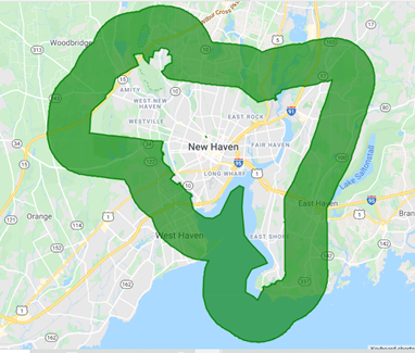
Fig. A1.5.9 A 2 km buffer around the original city boundary to serve as the rural reference
The use of a constant buffer assumes that all urban areas, regardless of size, have a similar influence around the city. This may not be true for large cities. In fact, there is some evidence that there is a footprint of the SUHI that is dependent on the size of the city (Yang et al. 2019, Zhou et al. 2015). As such, another way to define the buffered region is to normalize its area by the area of the urban cluster it surrounds (Chakraborty et al. 2021b, Peng et al. 2011). One way to do so in Earth Engine is by using an iterative method. This method (see code block below) uses functions to first calculate buffers of different widths around a geometry and then select the buffered region that is closest in size to the original geometry.
// Define sequence of buffer widths to be tested. |
Note how mapping the buff function over a sequence of pre-defined values, as done here, does not require loops, which are best avoided when using Earth Engine The same is true of mapping the bufferOptimize function: here it is mapped over a FeatureCollection with a single feature, but it would work even if regionInt contained multiple features. In this way, nested map functions in Earth Engine have the utility of nested loops in other languages.
Check the printed value on the Console. According to the result, within an uncertainty of 30 m, a buffer of 1170 m in width creates a polygon that is roughly equal to the area of the city. This function is best run via export when working with large feature collections.
The final way to define a rural reference does not use a buffer at all, but relies on land cover classes to select pixels that are urban versus non-urban (Chakraborty et al. 2020, Chakraborty and Lee 2019). For this, we will rely on the NLCD 2016 land cover data (Wickham et al. 2021) and create masks for urban and non-urban pixels (Fig. A1.5.10).
// Select the NLCD land cover data. |
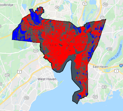
Fig. A1.5.10 Urban (red) and rural (blue) pixels in New Haven, Connecticut
We can then subsequently use these as masks to select urban versus rural LST pixels. You will find more about this in the next section.
Code Checkpoint A15d. The book’s repository contains a script that shows what your code should look like at this point.
Section 3. Calculating the Surface Urban Heat Island Intensity
Since the SUHI is the temperature difference between the urban area and the rural reference, we will calculate summary temperature values for the urban boundary and the different versions of rural reference using the Landsat and MODIS LST.
// Define function to reduce regions and summarize pixel values |
As you know from the code above, we extract urban temperature from MODIS ('MODIS_LST_urb) and from Landsat and MODIS ('MODIS_LST_urb_pix' and 'Landsat_LST_urb_pix') after considering only the urban pixels within the boundary.
Corresponding values are also extracted from the rural reference (including using only rural reference pixels within the urban boundary). For the buffered regions (both using constant width and variable width), we define and call another function.
// Define a function to reduce region and summarize pixel values |
We can print the newly created feature collections to go through these values for the different cases. Even though absolute MODIS and Landsat urban LSTs are different (29 for Landsat and 34 for MODIS), the SUHI is similar (3.6 C for MODIS and 4.8 C from Landsat). As one might expect, when only urban pixels are considered within the boundary, the average LST is higher (and lower for rural LST).
The SUHI variability within the city (Fig. A1.5.11) can then be displayed by subtracting the rural LST from the total LST:
// Display SUHI variability within the city. |
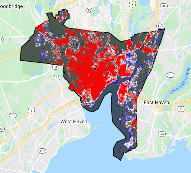
Fig. A1.5.11 Spatial variability in SUHI for the period of interest for New Haven, Connecticut. Red pixels show higher values and blue pixels show lower values.
Code Checkpoint A15e. The book’s repository contains a script that shows what your code should look like at this point.
Synthesis
Now that you know the different ways to calculate the SUHI and estimate LST using Earth Engine, load in your own city’s feature collection and compare the different methods.
Question 1. What are the SUHI values during summer and winter from the two products?
Question 2. How does a pixel-based urban-rural delineation method compare to a buffer-based method for SUHI estimation?
Conclusion
You should now have a good understanding of satellite measurements in the thermal bands, how they can be used to estimate LST, and how we can calculate the SUHI using these measurements.
Feedback
To review this chapter and make suggestions or note any problems, please go now to bit.ly/EEFA-review. You can find summary statistics from past reviews at bit.ly/EEFA-reviews-stats.
References
Cloud-Based Remote Sensing with Google Earth Engine. (n.d.). CLOUD-BASED REMOTE SENSING WITH GOOGLE EARTH ENGINE. https://www.eefabook.org/
Cloud-Based Remote Sensing with Google Earth Engine. (2024). In Springer eBooks. https://doi.org/10.1007/978-3-031-26588-4
Arnfield AJ (2003) Two decades of urban climate research: A review of turbulence, exchanges of energy and water, and the urban heat island. Int J Climatol 23:1–26. https://doi.org/10.1002/joc.859
Chakraborty TC, Lee X, Ermida S, Zhan W (2021) On the land emissivity assumption and Landsat-derived surface urban heat islands: A global analysis. Remote Sens Environ 265:112682. https://doi.org/10.1016/j.rse.2021.112682
Chakraborty TC, Sarangi C, Lee X (2021) Reduction in human activity can enhance the urban heat island: Insights from the COVID-19 lockdown. Environ Res Lett 16:54060. https://doi.org/10.1088/1748-9326/abef8e
Chakraborty T, Hsu A, Manya D, Sheriff G (2020) A spatially explicit surface urban heat island database for the United States: Characterization, uncertainties, and possible applications. ISPRS J Photogramm Remote Sens 168:74–88. https://doi.org/10.1016/j.isprsjprs.2020.07.021
Chakraborty T, Lee X (2019) A simplified urban-extent algorithm to characterize surface urban heat islands on a global scale and examine vegetation control on their spatiotemporal variability. Int J Appl Earth Obs Geoinf 74:269–280. https://doi.org/10.1016/j.jag.2018.09.015
Chakraborty T, Sarangi C, Tripathi SN (2017) Understanding diurnality and inter-seasonality of a sub-tropical urban heat island. Boundary-Layer Meteorol 163:287–309. https://doi.org/10.1007/s10546-016-0223-0
Clinton N, Gong P (2013) MODIS detected surface urban heat islands and sinks: Global locations and controls. Remote Sens Environ 134:294–304. https://doi.org/10.1016/j.rse.2013.03.008
Ermida SL, Soares P, Mantas V, et al (2020) Google Earth Engine open-source code for land surface temperature estimation from the Landsat series. Remote Sens 12:1471. https://doi.org/10.3390/RS12091471
Howard L (1833) The Climate of London: Deduced from Meteorological Observations Made in the Metropolis and at Various Places Around it. Harvey and Darton, J. and A. Arch, Longman, Hatchard, S. Highley and R. Hunter
Hu Y, Hou M, Jia G, et al (2019) Comparison of surface and canopy urban heat islands within megacities of eastern China. ISPRS J Photogramm Remote Sens 156:160–168. https://doi.org/10.1016/j.isprsjprs.2019.08.012
Kalnay E, Cai M (2003) Impact of urbanization and land-use change on climate. Nature 425:102. https://doi.org/10.1038/nature01952
Li K, Chen Y, Gao S (2022) Uncertainty of city-based urban heat island intensity across 1112 global cities: Background reference and cloud coverage. Remote Sens Environ 271:112898. https://doi.org/10.1016/j.rse.2022.112898
Li ZL, Wu H, Wang N, et al (2013) Land surface emissivity retrieval from satellite data. Int J Remote Sens 34:3084–3127. https://doi.org/10.1080/01431161.2012.716540
Malakar NK, Hulley GC, Hook SJ, et al (2018) An operational land surface temperature product for Landsat thermal data: Methodology and validation. IEEE Trans Geosci Remote Sens 56:5717–5735. https://doi.org/10.1109/TGRS.2018.2824828
Ngie A, Abutaleb K, Ahmed F, et al (2014) Assessment of urban heat island using satellite remotely sensed imagery: A review. South African Geogr J 96:198–214. https://doi.org/10.1080/03736245.2014.924864
Oke TR (1982) The energetic basis of the urban heat island. Q J R Meteorol Soc 108:1–24. https://doi.org/10.1002/qj.49710845502
Pekel JF, Cottam A, Gorelick N, Belward AS (2016) High-resolution mapping of global surface water and its long-term changes. Nature 540:418–422. https://doi.org/10.1038/nature20584
Peng S, Piao S, Ciais P, et al (2012) Surface urban heat island across 419 global big cities. Environ Sci Technol 46:6889–6890. https://doi.org/10.1021/es301811b
Qian Y, Chakraborty TC, Li J, et al (2022) Urbanization impact on regional climate and extreme weather: Current understanding, uncertainties, and future research directions. Adv Atmos Sci 39:819–860. https://doi.org/10.1007/s00376-021-1371-9
Sekertekin A, Bonafoni S (2020) Sensitivity analysis and validation of daytime and nighttime land surface temperature retrievals from Landsat 8 using different algorithms and emissivity models. Remote Sens 12:2776. https://doi.org/10.3390/RS12172776
Venter ZS, Chakraborty T, Lee X (2021) Crowdsourced air temperatures contrast satellite measures of the urban heat island and its mechanisms. Sci Adv 7:eabb9569. https://doi.org/10.1126/sciadv.abb9569
Wan Z (2006) MODIS land surface temperature products users’ guide. Inst Comput Earth Syst Sci Univ Calif St Barbar CA, USA 805
Wickham J, Stehman SV, Sorenson DG, et al (2021) Thematic accuracy assessment of the NLCD 2016 land cover for the conterminous United States. Remote Sens Environ 257:112357. https://doi.org/10.1016/j.rse.2021.112357
Yang Q, Huang X, Tang Q (2019) The footprint of urban heat island effect in 302 Chinese cities: Temporal trends and associated factors. Sci Total Environ 655:652–662. https://doi.org/10.1016/j.scitotenv.2018.11.171
Yao R, Wang L, Huang X, et al (2019) Greening in rural areas increases the surface urban heat island intensity. Geophys Res Lett 46:2204–2212. https://doi.org/10.1029/2018GL081816
Zhou D, Zhao S, Zhang L, et al (2015) The footprint of urban heat island effect in China. Sci Rep 5:1–11. https://doi.org/10.1038/srep11160