Cloud-Based Remote Sensing with Google Earth Engine
Fundamentals and Applications

Part F4: Interpreting Image Series
One of the paradigm-changing features of Earth Engine is the ability to access decades of imagery without the previous limitation of needing to download all the data to a local disk for processing. Because remote-sensing data files can be enormous, this used to limit many projects to viewing two or three images from different periods. With Earth Engine, users can access tens or hundreds of thousands of images to understand the status of places across decades.
Chapter F4.8: Data Fusion: Merging Classification Streams
Authors
Jeffrey A. Cardille, Rylan Boothman, Mary Villamor, Elijah Perez, Eidan Willis, Flavie Pelletier
Overview
As the ability to rapidly produce classifications of satellite images grows, it will be increasingly important to have algorithms that can sift through them to separate the signal from inevitable classification noise. The purpose of this chapter is to explore how to update classification time series by blending information from multiple classifications made from a wide variety of data sources. In this lab, we will explore how to update the classification time series of the Roosevelt River found in Fortin et al. (2020). That time series began with the 1972 launch of Landsat 1, blending evidence from 10 sensors and more than 140 images to show the evolution of the area until 2016. How has it changed since 2016? What new tools and data streams might we tap to understand the land surface through time?
Learning Outcomes
- Distinguishing between merging sensor data and merging classifications made from sensors.
- Working with the Bayesian Updating of Land Cover (BULC) algorithm, in its basic form, to blend classifications made across multiple years and sensors.
- Working with the BULC-D algorithm to highlight locations that changed.
Assumes you know how to:
- Import images and image collections, filter, and visualize (Part F1).
- Perform basic image analysis: select bands, compute indices, create masks, classify images (Part F2).
- Create a graph using ui.Chart (Chap. F1.3).
- Obtain accuracy metrics from classifications (Chap. F2.2).
Github Code link for all tutorials
This code base is collection of codes that are freely available from different authors for google earth engine.
Introduction to Theory
When working with multiple sensors, we are often presented with a challenge: What to do with classification noise? It’s almost impossible to remove all noise from a classification. Given the information contained in a stream of classifications, however, you should be able to use the temporal context to distinguish noise from true changes in the landscape.
The Bayesian Updating of Land Cover (BULC) algorithm (Cardille and Fortin 2016) is designed to extract the signal from the noise in a stream of classifications made from any number of data sources. BULC’s principal job is to estimate, at each time step, the likeliest state of land use and land cover (LULC) in a study area given the accumulated evidence to that point. It takes a stack of provisional classifications as input; in keeping with the terminology of Bayesian statistics, these are referred to as “Events,” because they provide new evidence to the system. BULC then returns a stack of classifications as output that represents the estimated LULC time series implied by the Events.
BULC estimates, at each time step, the most likely class from a set given the evidence up to that point in time. This is done by employing an accuracy assessment matrix like that seen in Chap. F2.2. At each time step, the algorithm quantifies the agreement between two classifications adjacent in time within a time series.
If the Events agree strongly, they are evidence of the true condition of the landscape at that point in time. If two adjacent Events disagree, the accuracy assessment matrix limits their power to change the class of a pixel in the interpreted time series. As each new classification is processed, BULC judges the credibility of a pixel’s stated class and keeps track of a set of estimates of the probability of each class for each pixel. In this way, each pixel traces its own LULC history, reflected through BULC’s judgment of the confidence in each of the classifications. The specific mechanics and formulas of BULC are detailed in Cardille and Fortin (2016).
BULC’s code is written in JavaScript, with modules that weigh evidence for and against change in several ways, while recording parts of the data-weighing process for you to inspect. In this lab, we will explore BULC through its graphical user interface (GUI), which allows rapid interaction with the algorithm’s main functionality.
Practicum
Section 1. Imagery and Classifications of the Roosevelt River
How has the Roosevelt River area changed in recent decades? One way to view the area’s recent history is to use Google Earth Timelapse, which shows selected annual clear images of every part of Earth’s terrestrial surface since the 1980s. (You can find the site quickly with a web search.) Enter “Roosevelt River, Brazil” in the search field. For centuries, this area was very remote from agricultural development. It was so little known to Westerners that when former US President Theodore Roosevelt traversed it in the early 1900s there was widespread doubt about whether his near-death experience there was exaggerated or even entirely fictional (Millard 2006). After World War II, the region saw increased agricultural development. Fortin et al. (2020) traced four decades of the history of this region with satellite imagery. Timelapse, meanwhile, indicates that land cover conversion continued after 2016. Can we track it using Earth Engine?
In this section, we will view the classification inputs to BULC, which were made separately from this lab exercise by identifying training points and classifying them using Earth Engine’s regression tree capability. As seen in Table 4.8.1, the classification inputs included Sentinel-2 optical data, Landsat 7, Landsat 8, and the Advanced Spaceborne Thermal Emission and Reflection Radiometer (ASTER) aboard Terra. Though each classification was made with care, they each contain noise, with each pixel likely to have been misclassified one or more times. This could lead us to draw unrealistic conclusions if the classifications themselves were considered as a time series. For example, we would judge it highly unlikely that an area represented by a pixel would really be agriculture one day and revert to intact forest later in the month, only to be converted to agriculture again soon after, and so on. With careful (though unavoidably imperfect) classifications, we would expect that an area that had truly been converted to agriculture would consistently be classified as agriculture, while an area that remained as forest would be classified as that class most of the time. BULC’s logic is to detect that persistence, extracting the true LULC change and stability from the noisy signal of the time series of classifications.
Table F4.8.1 Images classified for updating Roosevelt River LULC with BULC
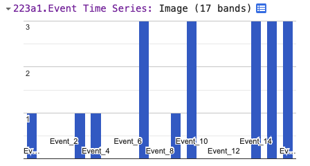
As you have seen in earlier chapters, creating classifications can be very involved and time consuming. To allow you to concentrate on BULC’s efforts to clean noise from an existing ImageCollection, we have created the classifications already and stored them as an ImageCollection asset. You can view the Event time series using the ui.Thumbnail function, which creates an animation of the elements of the collection. Paste the code below into a new script to see those classifications drawn in sequence in the Console.
var events=ee.ImageCollection( |
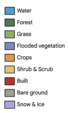
In the thumbnail sequence, the color palette shows Forest (class 1) as green, Water (class 2) as blue, and Active Agriculture (class 3) as yellow. Areas with no data in a particular Event are shown in black.
Code Checkpoint F48a. The book’s repository contains a script that shows what your code should look like at this point.
Section 2. Basics of the BULC Interface
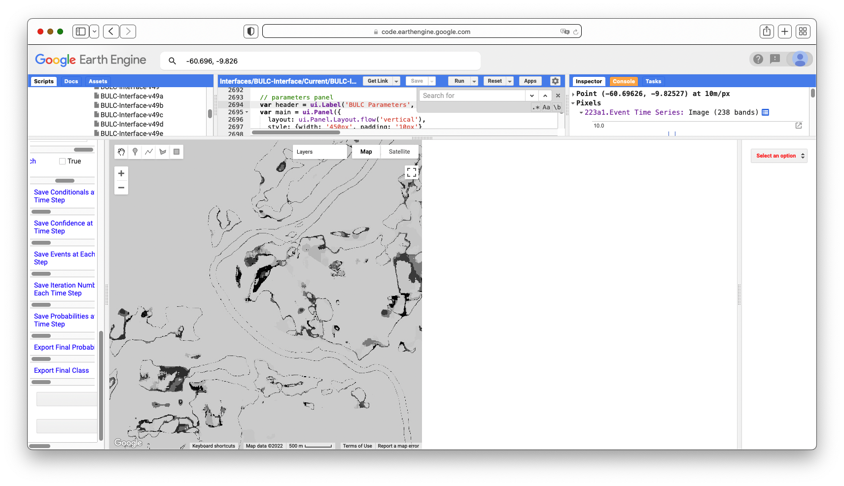
To see if BULC can successfully sift through these Events, we will use BULC’s GUI (Fig. F4.8.1), which makes interacting with the functionality straightforward. Code Checkpoint F48b in the book’s repository contains information about accessing that interface.
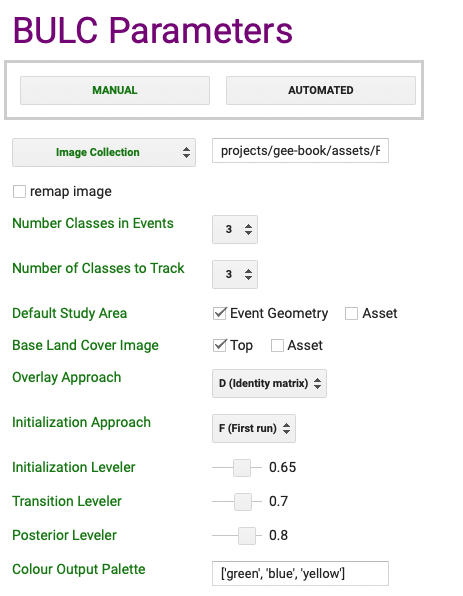
Fig. F4.8.1 BULC interface |

After you have run the script, BULC’s interface requires that a few parameters be set; these are specified using the left panel. Here, we describe and populate each of the required parameters, which are shown in red. As you proceed, the default red color will change to green when a parameter receives a value.
- The interface permits new runs to be created using the Manual or Automated methods. The Automated setting allows information from a previous run to be used without manual entry. In this tutorial, we will enter each parameter individually using the interface, so you should set this item to Manual by clicking once on it.
- Select type of image: The interface can accept pre-made Event inputs in one of three forms: (1) as a stored ImageCollection; (2) as a single multi-banded Image; and (3) as a stream of Dynamic World classifications. The classifications are processed in the order they are given, either within the ImageCollection or sequentially through the Image bands. For this run, select Image Collection from the dropdown menu, then enter the path to this collection, without enclosing it in quotes: projects/gee-book/assets/F4-8/cleanEvents
- Remap: in some settings, you might want to remap the input value to combine classes. Leave this empty for now; an example of this is discussed later in the lab.
- Number of Classes in Events and Number of Classes to Track: The algorithm requires the number of classes in each Event and the number of meaningful classes to track to be entered. Here, there are 3 classes in each classification (Forest, Water, and Active Agriculture) and 3 classes being tracked. (In the BULC-U version of the algorithm (Lee et al. 2018, 2020), these numbers may be different when the Events are made using unsupervised classifications, which may contain many more classes than are being tracked in a given run.) Meaningful classes are assumed by BULC to begin with 1 rather than 0, while class values of 0 in Events are treated as no data. As seen in the thumbnail of Events, there are 3 classes; set both of these values to 3.
- The Default Study Area is used by BULC to delimit the location to analyze. This value can be pulled from a specially sized Image or set automatically, using the extent of the inputs. Set this parameter to Event Geometry, which gets the value automatically from the Event collection.
- The Base Land Cover Image defines the initial land cover condition to which BULC adds evidence from Events. Here, we are working to update the land cover map from the end of 2016, as estimated in Fortin et al. (2020). The ending estimated classification from that study has been loaded as an asset and placed as the first image in the input ImageCollection. We will direct the BULC interface to use this first image in the collection as the base land cover image by selecting Top.
- Overlay Approach: BULC can run in multiple modes, which affect the outcome of the classification updating. One option, Overlay, overlays each consecutive Event with the one prior in the sequence, following Fortin et al. (2016). Another option, Custom, allows a user-defined constant array to be used. For this tutorial, we will choose D (Identity matrix), which uses the same transition table for every Event, regardless of how it overlays with the Event prior. That table gives a large conditional likelihood to the chance that classes agree strongly across the consecutive Event classifications that are used as inputs.
BULC makes relatively small demands on memory since its arithmetic uses only multiplication, addition, and division, without the need for complex function fitting. The specific memory use is tied to the overlay method used. In particular, Event-by-Event comparisons (the Overlay setting) are considerably more computationally expensive than pre-defined transition tables (the Identity and Custom settings). The maximum working Event depth is also slightly lowered when intermediate probability values are returned for inspection. Our tests indicate that with pre-defined truth tables and no intermediate probability values returned, BULC can handle updating problems hundreds of Events deep across an arbitrarily large area.
- Initialization Approach: If a BULC run of the full intended size ever surpassed the memory available, you would be able to break the processing into two or more parts using the following technique. First, create a slightly smaller run that can complete, and save the final probability image of that run. Because of the operation of Bayes’ theorem, the ending probability multi-band image can be used as the prior probability to continue processing Events with the same answers as if it had been run all at once. For this small run, we will select F (First Run).
- Levelers: BULC uses three levelers as part of its processing, as described in Fortin et al. (2016). The Initialization Leveler creates the initial probability vector of the initial LULC image; the Transition Leveler dampens transitions at each time step, making BULC less reactive to new evidence; and the Posterior Leveler ensures that each class retains nonzero probability so that the Bayes formula can function properly throughout the run. For this run, set the parameters to 0.65, 0.3, and 0.6, respectively. This corresponds to a typical set of values that is appropriate when moderate-quality classifications are fed to BULC.
- Colour Output Palette: We will use the same color palette as what was seen in the small script you used to draw the Events, with one exception. Because BULC will give a value for the estimated class for every pixel, there are no pixels in the study area with missing or masked data. To line up the colors with the attainable numbers, we will remove the color ‘black’ from the specification. For this field, enter this list: ['green', 'blue', 'yellow']. For all of the text inputs, make sure to click outside that field after entering text so that the input information is registered; the changing of the text color to green confirms that the information was received.
When you have finished setting the required parameters, the interface will look like Fig. 4.8.2.
Fig. 4.8.2 Initial settings for the key driving parameters of BULC |
Beneath the required parameters is a set of optional parameters that affect which intermediate results are stored during a run for later inspection. We are also given a choice of returning intermediate results for closer inspection. At this stage, you can leave all optional parameters out of the BULC call by leaving them blanked or unchecked.
After clicking the Apply Parameters button at the bottom of the left panel, the classifications and parameters are sent to the BULC modules. The Map will move to the study area, and after a few seconds, the Console will hold new thumbnails. The uppermost thumbnail is a rapidly changing view of the input classifications. Beneath that is a thumbnail of the same area as interpreted by BULC. Beneath those is a Confidence thumbnail, which is discussed in detail later in this lab.
The BULC interpretation of the landscape looks roughly like the Event inputs, but it is different in two important ways. First, depending on the leveler settings, it will usually have less noise than the Event classifications. In the settings above, we used the Transition and Posterior levelers to tell BULC to trust past accumulated evidence more than a single new image. The second key difference between the BULC result and the input classifications is that even when the inputs don’t cover the whole area at each time step, BULC provides an estimate in every pixel at each time step. To create this continuous classification, if a new classification does not have data for some part of the study area (beyond the edge of a given image, for example), the last best guess from the previous iteration is carried forward. Simply put, the estimate in a given pixel is kept the same until new data arrives.
Meanwhile, below the Console, the rest of the interface changes when BULC is run. The Map panel displays BULC’s classification for the final date: that is, after considering the evidence from each of the input classifications. We can use the Satellite background to judge whether BULC is accurately capturing the state of LULC. This can be done by unselecting the drawn layers in the map layer set and selecting Satellite from the choices in the upper-right part of the Map panel. Earth Engine’s background satellite images are often updated, so you should see something like the right side of Fig. F4.8.3, though it may differ slightly.
Fig. 4.8.3 BULC estimation of the state of LULC at the end of 2021 (left). Satellite backdrop for Earth Engine (right), which may differ from what you see due to updates. |


Question 1. When comparing the BULC classification for 2021 against the current Earth Engine satellite view, what are the similarities and differences? Note that in Earth Engine, the copyrighted year numbers at the bottom of the screen may not coincide with the precise date of the image shown.
In the rightmost panel below the Console, the interface offers you multiple options for viewing the results. These include:
- Movie. This uses the ui.Thumbnail API function to draw the BULC results rapidly in the viewer. This option offers you a control on the frame rate (in frames per second), and a checkbox affecting the drawing resolution. The high-resolution option uses the maximum resolution permitted given the function’s constraints. A lower resolution setting constructs the thumbnail more quickly, but at a loss of detail.
- Filmstrip. This produces an image like the Movie option, but allows you to move on request through each image.
- Mosaic. This draws every BULC result in the panel. Depending on the size of the stack of classifications, this could become quite a large set of images.
- Zoom. This draws the final BULC classification at multiple scales, with the finest-scale image matching that shown in the Map window.
Question 2. Select the BULC option, then select the Movie tool to view the result, and choose a drawing speed and resolution. When viewing the full area, would you assess the additional LULC changes since 2016 as being minor, moderate, or major compared to the changes that occurred before 2016? Explain the reasoning for your assessment.
Section 3. Detailed LULC Inspection with BULC
BULC results can be viewed interactively, allowing you to view more detailed estimations of the LULC around the study area. We will zoom into a specific area where change did occur after 2016. To do that, turn on the Satellite view and zoom in. Watching the scale bar in the lower right of the Map panel, continue zooming until the scale bar says 5 km. Then, enter "-60.742, -9.844" in the Earth Engine search tool, located above the code. The text will be interpreted as a longitude/latitude value and will offer you a nearby coordinate, indicated with a value for the degrees West and the degrees South. Click that entry and Earth Engine will move to that location, while keeping at the specified zoom level. Let’s compare the BULC result in this sector against the image from Earth Engine’s satellite view that is underneath it (Fig. 4.8.4).
Fig. 4.8.4 Comparison of the final classification of the northern part of the study area to the satellite view |


BULC captured the changes between 2016 and 2021 with a classification series that suggests agricultural development (Fig. 4.8.4, left). Given the appearance of BULC’s 2021 classification, it suggests that the satellite backdrop at the time of this writing (Fig. 4.8.4, right) came from an earlier time period.
Now, in the Results panel, select BULC, then Movie. Set your desired frame speed and resolution, then select Redraw Thumbnail. Then, zoom the main Map even closer to some agriculture that appears to have been established between 2016 and 2021. Redraw the thumbnail movie as needed to find an interesting set of pixels.
With this finer-scale access to the results of BULC, you can select individual pixels to inspect. Move the horizontal divider downward to expose the Inspector tab and Console tab. Use the Inspector to click on several pixels to learn their history as expressed in the inputted Events and in BULC’s interpretation of the noise and signal in the Event series. In a chosen pixel, you might see output that looks like Fig. 4.8.5. It indicates a possible conversion in the Event time series after a few classifications of the pixel as Forest. This decreases the confidence that the pixel is still Forest (Fig. 4.8.5, lower panel), but not enough for the Active Agriculture class (class 3) to become the dominant probability. After the subsequent Event labels the pixel as Forest, the confidence (lower panel) recovers slightly, but not to its former level. The next Event classifies the pixel as Active Agriculture, confidently, by interpreting that second Active Agriculture classification, in a setting where change was already somewhat suspected after the first non-Forest classification. BULC’s label (middle panel) changes to be Active Agriculture at that point in the sequence. Subsequent Event classifications as Active Agriculture creates a growing confidence that its proper label at the end of the sequence was indeed Active Agriculture.
Fig. 4.8.5 History for 2016-2020 for a pixel that appeared to have been newly cultivated during that period. (above): the input classifications, which s |


Question 3. Run the code again with the same data, but adjust the three levelers, then view the results presented in the Map window and the Results panel. How do each of the three parameters affect the behavior of BULC in its results? Use the thumbnail to assess your subjective satisfaction with the results, and use the Inspector to view the BULC behavior in individual pixels. Can you produce an optimal outcome for this given set of input classifications?
Section 4. Change Detection with BULC-D
What if we wanted to identify areas of likely change or stability without trying to identify the initial and final LULC class? BULC-D is an algorithm that estimates, at each time step, the probability of noteworthy change. The example below uses the Normalized Burn Ratio (NBR) as a gauge: BULC-D assesses whether the ratio has meaningfully increased, decreased, or remained the same. It is then the choice of the analyst to decide how to treat these assessed probabilities of stability and change.
BULC-D involves determining an expectation for an index across a user-specified time period and then comparing new values against that estimation. Using Bayesian logic, BULC-D then asks which of three hypotheses is most likely, given evidence from the new values to date from that index. The hypotheses are simple: Either the value has decreased meaningfully, or it has increased meaningfully, or it has not changed substantially compared to the previously established expectation. The details of the workings of BULC-D are beyond the scope of this exercise, but we provide it as a tool for exploration. BULC-D’s basic framework is the following:
- Establish: Fit a harmonic curve with a user-specified number of terms to a stream of values from an index, such as the Normalized Difference Vegetation Index (NDVI), NBR, etc.
- Standardize: For each new image, quantify the deviation of the index’s value from the expectation on that date.
- Contextualize: Assess the magnitude of that deviation in one of several ordered bins.
- Synthesize: Use the BULC framework to adjust the vector of change for the three possibilities: the value went down, the value stayed the same, the value went up.
It is worth noting that BULC-D does not label the change with a LULC category; rather, it trains itself to distinguish likely LULC change from expected variability. In this way, BULC-D can be thought of as a “sieve” through which you are able to identify locations of possible change, isolated from likely background noise. In the BULC-D stage, the likeliness of change is identified across the landscape; in a separate second stage, the meaning of those changes and any changes to LULC classes are identified. We will explore the workings of BULC-D using its GUI.
Code Checkpoint F48c. The book’s repository contains information about accessing that interface.
After you have run the script to initialize the interface, BULC-D’s interface requires a few parameters to be set. For this run of BULC-D, we will set the parameters to the following:
- Expectation years: 2020
- Target year: 2021
- Sensors: Landsat and Sentinel
- Index: NBR
- Harmonic fit: Yes, 1 harmonic term.
Run BULC-D for this area. As a reminder, you should first zoom in enough that the scale bar reads “5 km” or finer. Then, search for the location "-60.7624, -9.8542". When you run BULC-D, a result like Fig. F4.8.6 is shown for the layer of probabilities.
|
Fig. 4.8.6 Result for BULC-D for the Roosevelt River area, depicting estimated probability of change and stability for 2021 |
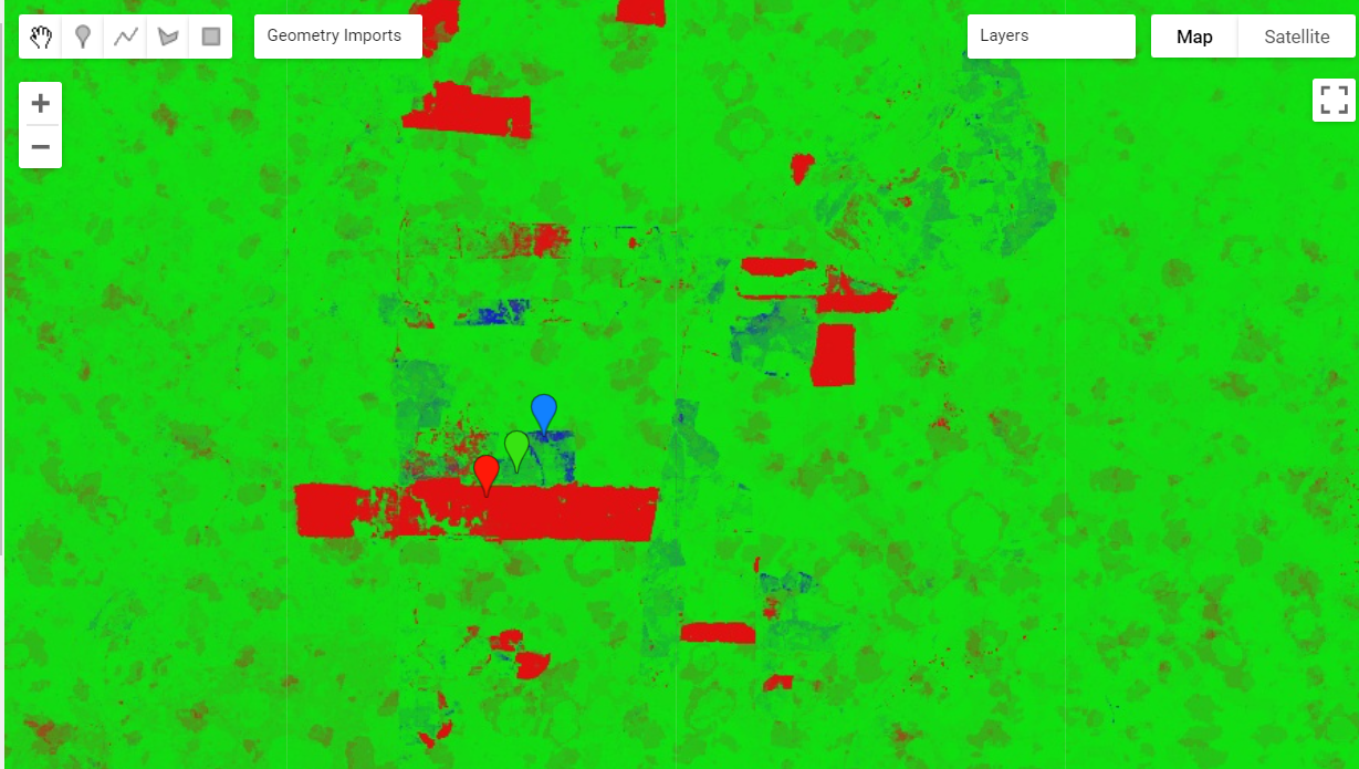
The BULC-D image (Fig. F4.8.6) shows each pixel as a continuous three-value vector along a continuous range; the three values sum to 1. For example, a vector with values of [0.85, 0.10, 0.05] would represent an area estimated with high confidence according to BULC-D to have experienced a sustained drop in NBR in the target period compared to the values set by the expectation data. In that pixel, the combination of three colors would produce a value that is richly red. You can see Chap. F1.1 for more information on drawing bands of information to the screen using the red-green-blue additive color model in Earth Engine.
Each pixel experiences its own NBR history in both the expectation period and the target year. Next, we will highlight the history of three nearby areas: one, marked with a red balloon in your interface, that BULC assessed as having experienced a persistent drop in NBR; a second in green assessed to not have changed, and a third in blue assessed to have witnessed a persistent NBR increase.
Figure F4.8.7 shows the NBR history for the red balloon in the southern part of the study area in Fig. F4.8.4. If you click on that pixel or one like it, you can see that, whereas the values were quite stable throughout the growing season for the years used to create the pixel’s expectation, they were persistently lower in the target year. This is flagged as a likely meaningful drop in the NBR by BULC-D, for consideration by the analyst.
|
Fig. 4.8.7 NBR history for a pixel with an apparent drop in NBR in the target year (below) as compared to the expectation years (above). Pixel is colored a shade of red in Fig. 4.8.6. |
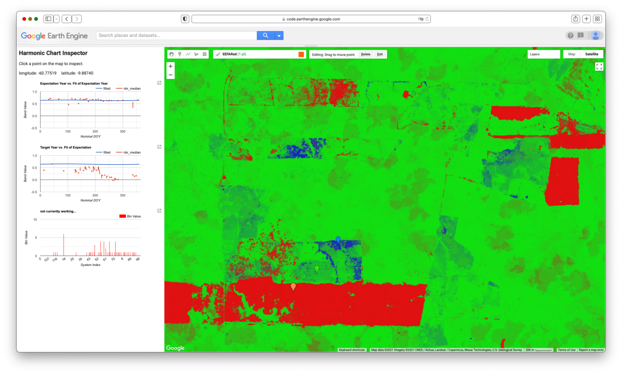
Figure F4.8.8 shows the NBR history for the blue balloon in the southern part of the study area in Fig. F4.8.4. For that pixel, while the values were quite stable throughout the growing season for the years used to create the pixel’s expectation, they were persistently higher in the target year.
Question 4. Experiment with turning off one of the satellite sensor data sources used to create the expectation collection. For example, do you get the same results if the Sentinel-2 data stream is not used, or is the outcome different. You might make screen captures of the results to compare with Fig. 4.8.4. How strongly does each satellite stream affect the outcome of the estimate? Do differences in the resulting estimate vary across the study area?
Fig. 4.8.8 NBR history for a pixel with an apparent increase in NBR in the target year (below) as compared to the expectation years (above). Pixel is colored a shade of blue in Fig. 4.8.6. |

Figure F4.8.8 also shows that, for that pixel, the fit of values for the years used to build the expectation showed a sine wave (shown in blue), but with a fit that was not very strong. When data for the target year was assembled (Fig. F4.8.8, bottom), the values were persistently above expectation throughout the growing season. Note that this pixel was identified as being different in the target year as compared to earlier years, which does not rule out the possibility that the LULC of the area was changed (for example, from Forest to Agriculture) during the years used to build the expectation collection. BULC-D is intended to be run steadily over a long period of time, with the changes marked as they occur, after which point the expectation would be recalculated.
Fig. 4.8.9 NBR history for a pixel with no apparent increase or decrease in NBR in the target year (below) as compared to the expectation years (above). Pixel is colored a shade of green in Fig. 4.8.6. |
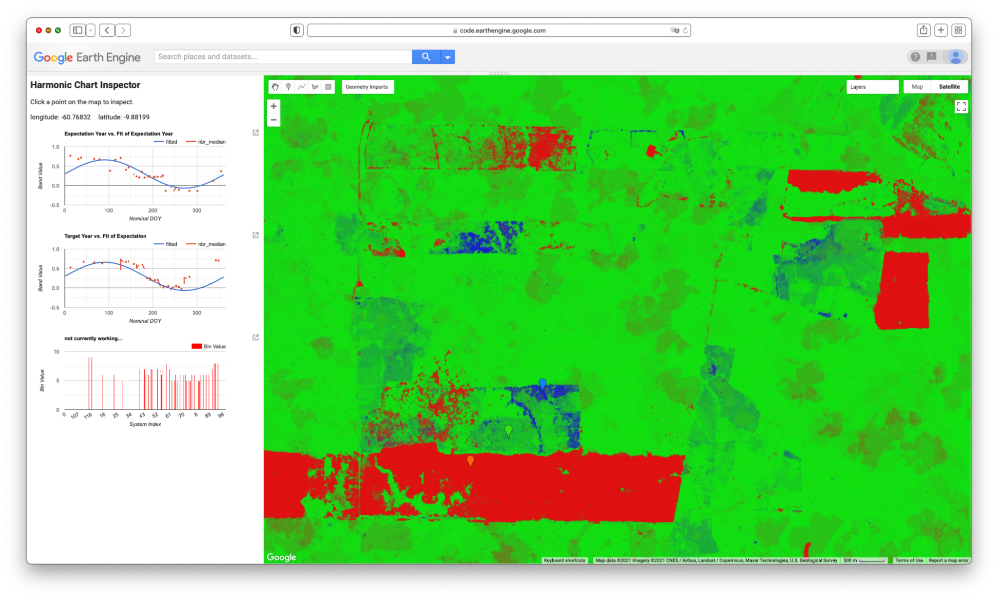
Fig. F4.8.9 shows the NBR history for the green balloon in the southern part of the study area in Fig. F4.8.4. For that pixel, the values in the expectation collection formed a sine wave, and the values in the target collection deviated only slightly from the expectation during the target year.
Section 5. Change Detection with BULC and Dynamic World
Recent advances in neural networks have made it easier to develop consistent models of LULC characteristics using satellite data. The Dynamic World project (Brown et al. 2022) applies a neural network, trained on a very large number of images, to each new Sentinel-2 image soon after it arrives. The result is a near-real-time classification interpreting the LULC of Earth’s surface, kept continually up to date with new imagery.
What to do with the inevitable inconsistencies in a pixel’s stated LULC class through time? For a given pixel on a given image, its assigned class label is chosen by the Dynamic World algorithm as the maximum class probability given the band values on that day. Individual class probabilities are given as part of the dataset and could be used to better interpret a pixel’s condition and perhaps its history. Future work with BULC will involve incorporating these probabilities into BULC’s probability-based structure. For this tutorial, we will explore the consistency of the assigned labels in this same Roosevelt River area as a way to illustrate BULC’s potential for minimizing noise in this vast and growing dataset.
5.1. Using BULC To Explore and Refine Dynamic World Classifications
Code Checkpoint A48d. The book’s repository contains a script to use to begin this section. You will need to load the linked script and run it to begin.
After running the linked script, the BULC interface will initialize. Select Dynamic World from the dropdown menu where you earlier selected Image Collection. When you do, the interface opens several new fields to complete. BULC will need to know where you are interested in working with Dynamic World, since it could be anywhere on Earth. To specify the location, the interface field expects a nested list of lists of lists, which is modeled after the structure used inside the constructor ee.Geometry.Polygon. (When using drawing tools or specifying study areas using coordinates, you may have noticed this structure.) Enter the following nested list in the text field near the Dynamic World option, without enclosing it in quotes:
[[[-61.155, -10.559], [-60.285, -10.559], [-60.285, -9.436], [-61.155, -9.436]]] |
Next, BULC will need to know which years of Dynamic World you are interested in. For this exercise, select 2021. Then, BULC will ask for the Julian days of the year that you are interested in. For this exercise, enter 150 for the start day and 300 for the end day. Because you selected Dynamic World for analysis in BULC, the interface defaults to offering the number 9 for the number of classes in Events and for the number of classes to track. This number represents the full set of classes in the Dynamic World classification scheme. You can leave other required settings shown in green with their default values. For the Color Output Palette, enter the following palette without quotes. This will render results in the Dynamic World default colors.
['419BDF', '397D49', '88B053' |
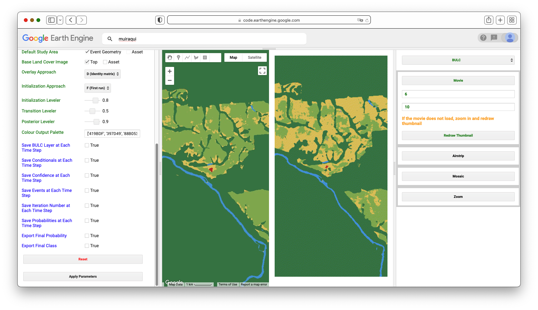
When you have finished, select Apply Parameters at the bottom of the input panel. When it runs, BULC subsets the Dynamic World dataset to clip out according to the dates and location, identifying images from more than 40 distinct dates. The area covers two of the tiles in which Dynamic World classifications are partitioned to be served, so BULC receives more than 90 classifications. When BULC finishes its run, the Map panel will look like Fig. F4.8.10, BULC’s estimate of the final state of the landscape at the end of the classification sequence.
Fig. F4.8.10 BULC classification using default settings for Roosevelt River area for late 2021 |

Let’s explore the suite of information returned by BULC about this time period in Dynamic World. Enter “Muiraquitã” in the search bar and view the results around that area to be able to see the changing LULC classifications within farm fields. Then, begin to inspect the results by viewing a Movie of the Events, with a data frame rate of 6 frames per second. Because the study area spans multiple Dynamic World tiles, you will find that many Event frames are black, meaning that there was no data in your sector on that particular image. Because of this, and also perhaps because of the very aggressive cloud masking built into Dynamic World, viewing Events (which, as a reminder, are the individual classified images directly from Dynamic World) can be a very challenging way to look for change and stability. BULC’s goal is to sift through those classifications to produce a time series that reflects, according to its estimation, the most likely LULC value at each time step. View the Movie of the BULC results and ask yourself whether each class is equally well replicated across the set of classifications. A still from midway through the Movie sequence of the BULC results can be seen in Fig. F4.8.11.
Fig. F4.8.11 Still frame (right image) from the animation of BULC’s adjusted estimate of LULC through time near Muiraquitã |
As BULC uses the classification inputs to estimate the state of the LULC at each time step, it also tracks its confidence in those estimates. This is shown in several ways in the interface.
- You can view a Movie of BULC’s confidence through time as it reacts to the consistency or variability of the class identified in each pixel by Dynamic World. View that movie now over this area to see the evolution of BULC’s confidence through time of the class of each pixel. A still frame from this movie can be seen in Fig. F4.8.12. The frame and animation indicate that BULC’s confidence is lowest in pixels where the estimate flips between similar categories, such as Grass and Shrub & Scrub. It also is low at the edges of land covers, even where the covers (such as Forest and Water) are easy to discern from each other.
- You can inspect the final confidence estimate from BULC, which is shown as a grayscale image in the set of Map layers in the left lower panel. That single layer synthesizes how, across many Dynamic World classifications, the confidence in certain LULC classes and locations is ultimately more stable than in others. For example, generally speaking, the Forest class is classified consistently across this assemblage of Dynamic World images. Agriculture fields are less consistently classified as a single class, as evidenced by their relatively low confidence.
- Another way of viewing BULC’s confidence is through the Inspector tab. You can click on individual pixels to view their values in the Event time series and in the BULC time series, and see BULC’s corresponding confidence value changing through time in response to the relative stability of each pixel’s classification.
- Another way to view BULC’s confidence estimation is as a hillshade enhancement of the final BULC classification. If you select the Probability Hillshade in the set of Map layers, it shows the final BULC classification as a textured surface, in which you can see where lower-confidence pixels are classified.
Fig. F4.8.12 Still frame from the animation of changing confidence through time, near Muiraquitã. |

5.2. Using BULC To Visualize Uncertainty of Dynamic World in Simplified Categories
In the previous section, you may have noticed that there are two main types of uncertainty in BULC’s assessment of long-term classification confidence. One type is due to spatial uncertainty at the edge of two relatively distinct phenomena, like the River/Forest boundary visible in Fig. F4.8.12. These are shown in dark tones in the confidence images, and emphasized in the Probability Hillshade. The other type of uncertainty is due to some cause of labeling uncertainty, due either (1) to the similarity of the classes, or (2) to persistent difficulty in distinguishing two distinct classes that are meaningfully different but spectrally similar. An example of uncertainty due to similar labels is distinguishing flooded and non-flooded wetlands in classifications that contain both those categories. An example of difficulty distinguishing distinct but spectrally similar classes might be distinguishing a parking lot from a body of water.
BULC allows you to remap the classifications it is given as input, compressing categories as a way to minimize uncertainty due to similarity among classes. In the setting of Dynamic World in this study area, we notice that several classes are functionally similar for the purposes of detecting new deforestation: Farm fields and pastures are variously labeled on any given Dynamic World classification as Grass, Flooded Vegetation, Crops, Shrub & Scrub, Built, or Bare Ground. What if we wanted to combine these categories to be similar to the distinctions of the classified Events from this lab’s Sect. 1? The classes in that section were Forest, Water, and Active Agriculture. To remap the Dynamic World classification, continue with the same run as in Sect. 5.1. Near where you specified the location for clipping Dynamic World, there are two fields for remapping. Select the Remap checkbox and in the “from” field, enter (without quotes):
0,1,2,3,4,5,6,7,8
In the “to” field, enter (without quotes):
1,0,2,2,2,2,2,2,0
This directs BULC to create a three-class remap of each Dynamic World image. Next, in the area of the interface where you specify the palette, enter the same palette used earlier:
['green', 'blue', 'yellow']
Before continuing, think for a moment about how many classes you have now. From BULC’s perspective, the Dynamic World events will have 3 classes and you will be tracking 3 classes. Set both the Number of Classes in Events and Number of Classes to Track to 3. Then click Apply Parameters to send this new run to BULC.
The confidence image shown in the main Map panel is instructive (Fig. 4.8.13). Using data from 2020, 2021, and 2022, It indicates that much of the uncertainty among the original Dynamic World classifications was in distinguishing labels within agricultural fields. When that uncertainty is removed by combining classes, the BULC result indicates that a substantial part of the remaining uncertainty is at the edges of distinct covers. For example, in the south-central and southern part of the frame, much of the uncertainty among classifications in the original Dynamic World classifications was due to distinction among the highly similar, easily confused classes. Much of what remained (right) after remapping (right) formed outlines of the river and the edges between farmland and forest: a graphic depiction of the “spatial uncertainty” discussed earlier. Yet not all of the uncertainty was spatial; the thicker, darker areas of uncertainty even after remapping (right, at the extreme eastern edge for example) indicates a more fundamental disagreement in the classifications. In those pixels, even when the Agriculture-like classes were compressed, there was still considerable uncertainty (likely between Forest and Active Agriculture) in the true state of these areas. These might be of further interest: were they places newly deforested in 2020-2022? Were they abandoned fields regrowing? Were they degraded at some point? The mapping of uncertainty may hold promise for a better understanding of uncertainty as it is encountered in real classifications, thanks to Dynamic World.
Fig. F4.8.13 Final confidence layer from the run with (left) and without (right) remapping to combine similar LULC classes to distinguish Forest, Water, and Active Agriculture near -60.696W, -9.826S |

Given the tools and approaches presented in this lab, you should now be able to import your own classifications for BULC (Sects. 1–3), detect changes in sets of raw imagery (Sect. 4), or use Dynamic World’s pre-created classifications (Sect. 5). The following exercises explore this potential.
Synthesis
Assignment 1. For a given set of classifications as inputs, BULC uses three parameters that specify how strongly to trust the initial classification, how heavily to weigh the evidence of each classification, and how to adjust the confidence at the end of each time step. For this exercise, adjust the values of these three parameters to explore the strength of the effect they can have on the BULC results.
Assignment 2. The BULC-D framework produces a continuous three-value vector of the probability of change at each pixel. This variability accounts for the mottled look of the figures when those probabilities are viewed across space. Use the Inspector tool or the interface to explore the final estimated probabilities, both numerically and as represented by different colors of pixels in the given example. Compare and contrast the mean NBR values from the earlier and later years, which are drawn in the Layer list. Then answer the following questions:
- In general, how well does BULC-D appear to be identifying locations of likely change?
- Does one type of change (decrease, increase, no change) appear to be mapped better than the others? If so, why do you think this is?
Assignment 3. The BULC-D example used here was for 2021. Run it for 2022 or later at this location. How well do results from adjacent years complement each other?
Assignment 4. Run BULC-D in a different area for a year of interest of your choosing. How do you like the results?
Assignment 5. Describe how you might use BULC-D as a filter for distinguishing meaningful change from noise. In your answer, you can consider using BULC-D before or after BULC or some other time-series algorithm, like CCDC or LandTrendr.
Assignment 6. Analyze stability and change with Dynamic World for other parts of the world and for other years. For example, you might consider:
- Quebec, Canada, days 150–300 for 2019 and 2020:
[[[-71.578, 49.755], [-71.578, 49.445], [-70.483, 49.445], [-70.483, 49.755]]]
Location of a summer 2020 fire
- Addis Ababa, Ethiopia: [[[38.79, 9.00], [38.79, 8.99], [38.81, 8.99], [38.81, 9.00]]]
- Calacalí, Ecuador: [[[-78.537, 0.017], [-78.537, -0.047], [-78.463, -0.047], [-78.463, 0.017]]]
- Irpin, Ukraine: [[[30.22, 50.58], [30.22, 50.525], [30.346, 50.525], [30.346, 50.58]]]
- A different location of your own choosing. To do this, use the Earth Engine drawing tools to draw a rectangle somewhere on Earth. Then, at the top of the Import section, you will see an icon that looks like a sheet of paper. Click that icon and look for the polygon specification for the rectangle you drew. Paste that into the location field for the Dynamic World interface.
Conclusion
In this lab, you have viewed several related but distinct ways to use Bayesian statistics to identify locations of LULC change in complex landscapes. While they are standalone algorithms, they are each intended to provide a perspective either on the likelihood of change (BULC-D) or of extracting signal from noisy classifications (BULC). You can consider using them especially when you have pixels that, despite your best efforts, periodically flip back and forth between similar but different classes. BULC can help ignore noise, and BULC-D can help reveal whether this year’s signal has precedent in past years.
To learn more about the BULC algorithm, you can view this interactive probability illustration tool by a link found in script F48s1 - Supplemental in the book's repository. In the future, after you have learned how to use the logic of BULC, you might prefer to work with the JavaScript code version. To do that, you can find a tutorial at the website of the authors.
Feedback
To review this chapter and make suggestions or note any problems, please go now to bit.ly/EEFA-review. You can find summary statistics from past reviews at bit.ly/EEFA-reviews-stats.
References
Cloud-Based Remote Sensing with Google Earth Engine. (n.d.). CLOUD-BASED REMOTE SENSING WITH GOOGLE EARTH ENGINE. https://www.eefabook.org/
Cloud-Based Remote Sensing with Google Earth Engine. (2024). In Springer eBooks. https://doi.org/10.1007/978-3-031-26588-4
Brown CF, Brumby SP, Guzder-Williams B, et al (2022) Dynamic World, Near real-time global 10 m land use land cover mapping. Sci Data 9:1–17. https://doi.org/10.1038/s41597-022-01307-4
Cardille JA, Fortin JA (2016) Bayesian updating of land-cover estimates in a data-rich environment. Remote Sens Environ 186:234–249. https://doi.org/10.1016/j.rse.2016.08.021
Fortin JA, Cardille JA, Perez E (2020) Multi-sensor detection of forest-cover change across 45 years in Mato Grosso, Brazil. Remote Sens Environ 238. https://doi.org/10.1016/j.rse.2019.111266
Lee J, Cardille JA, Coe MT (2020) Agricultural expansion in Mato Grosso from 1986-2000: A Bayesian time series approach to tracking past land cover change. Remote Sens 12. https://doi.org/10.3390/rs12040688
Lee J, Cardille JA, Coe MT (2018) BULC-U: Sharpening resolution and improving accuracy of land-use/land-cover classifications in Google Earth Engine. Remote Sens 10. https://doi.org/10.3390/rs10091455
Millard C (2006) The River of Doubt: Theodore Roosevelt’s Darkest Journey. Anchor