Cloud-Based Remote Sensing with Google Earth Engine

Fundamentals and Applications

Part A3: Terrestrial Applications

Earth’s terrestrial surface is analyzed regularly by satellites, in search of both change and stability. These are of great interest to a wide cross-section of Earth Engine users, and projects across large areas illustrate both the challenges and opportunities for life on Earth. Chapters in this Part illustrate the use of Earth Engine for disturbance, understanding long-term changes of rangelands, and creating optimum study sites.

Chapter A3.7: Creating Presence and Absence Points

Authors

Peder Engelstad, Daniel Carver, Nicholas E. Young

Overview 

The purpose of this chapter is to demonstrate a method to generate your own presence and absence data and distribute those samples using specific ecological characteristics found in remotely sensed imagery. You will see that even when field data is unavailable, you can still digitally sample a landscape and gather information on current or past ecological conditions.

Learning Outcomes

• Generating presence and absence data manually using high-resolution imagery.
• Generating randomly distributed points automatically within a feature class layer to use as field sampling locations.
• Filtering your points to refine your sampling locations.

Helps if you know how to:

• Import images and image collections, filter, and visualize (Part F1).
• Visualize images with a variety of false-color band combinations (Chap. F1.1).
• Perform basic image analysis: select bands, compute indices, create masks (Part F2).
• Use normalizedDifference to calculate vegetation indices (Chap. F2.0).
• Use drawing tools to create points, lines, and polygons (Chap. F2.1).
• Filter a FeatureCollection to obtain a subset (Chap. F5.0, Chap. F5.1).

Github Code link for all tutorials

This code base is collection of codes that are freely available from different authors for google earth engine.

Github Source

Introduction to Theory

Herbivore grazing can have a negative effect on aspen regeneration in some areas, as aspens tend to grow in large monotypic stands (Halofsky and Ripple 2008). Excluding elk, deer, and cow grazing from an area has observable effects on aspen regrowth. In a hypothetical study, we may be interested in understanding the effect of herbivory from these species on various ecological aspects of aspen stands. But how can we monitor aspen stands without setting foot in the field? In this chapter, we will use multiple datasets and high-resolution resolution imagery (1 m2) to generate sampling locations for this theoretical field survey. We will also build a presence/absence dataset that could be used to train a spatial model of aspen coverage.

Practicum

The National Land Cover Database (NLCD) is a Landsat-derived land cover database with 30 m spatial resolution, available at multiple time periods. Data from 1992 are primarily based on an unsupervised classification of Landsat data. The other years rely on a decision-tree classification to identify the land cover classes.

The National Agriculture Imagery Program (NAIP) acquires aerial imagery during the agricultural growing seasons across the continental United States. NAIP projects are contracted each year based upon available funding and the Farm Service Agency imagery acquisition cycle. NAIP imagery is acquired at a one-meter ground sample distance with a horizontal accuracy that matches within six meters of photo-identifiable ground control points. NAIP imagery is often collected in four bands: blue, green, red, and near infrared. The near infrared band is helpful in distinguishing between different types of vegetation.

The USGS National Elevation Dataset (NED) 1/3 arc-second is an elevation dataset produced by the USGS. This coast-to-coast dataset is available at 0.33 arc-second spatial resolution (30 m) across the lower 48 states, parts of Alaska, Hawaii, and US Territories.

Section 1. Developing Your Own Sampling Locations

We will start by developing potential field sampling locations based on the relative physical and ecological conditions.

Section 1.1. Region of Interest

The geographic region for this chapter is the Grand Mesa in western Colorado. Considered to be the largest mesa in the world by area, the Grand Mesa rises from 4000 feet near Grand Junction, Colorado, to over 10000 feet at its highest point. Historically, the Grand Mesa was glaciated, leaving its top flattened and spotted with lakes. While heavily forested at higher elevation, there are distinct transitions between shrubland, aspen, and conifer forest along the steep slopes. As one of the westernmost extensions of the montane environment in Colorado, the Grand Mesa represents important habitat for many ungulate species.

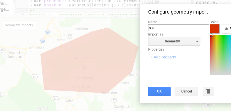
Our first step is to open a new script in Earth Engine. First, create a region of interest that encompasses the Grand Mesa (you can search for it by name in the search bar at the top). Do so using the geometry tool. Once you create the feature, rename it roi (Fig. A3.7.1).

Section 1.2. Working with NAIP

We will rely on NAIP imagery for multiple steps in this process. NAIP imagery is not collected every year, so it makes sense to load in multiple years to determine what time frame is available. We will use a print statement to see what years are available for our area from 2015 and 2017. Copy the following code to start your script.

When you run the script you will see a print statement similar to the one shown in Fig. A3.7.2.

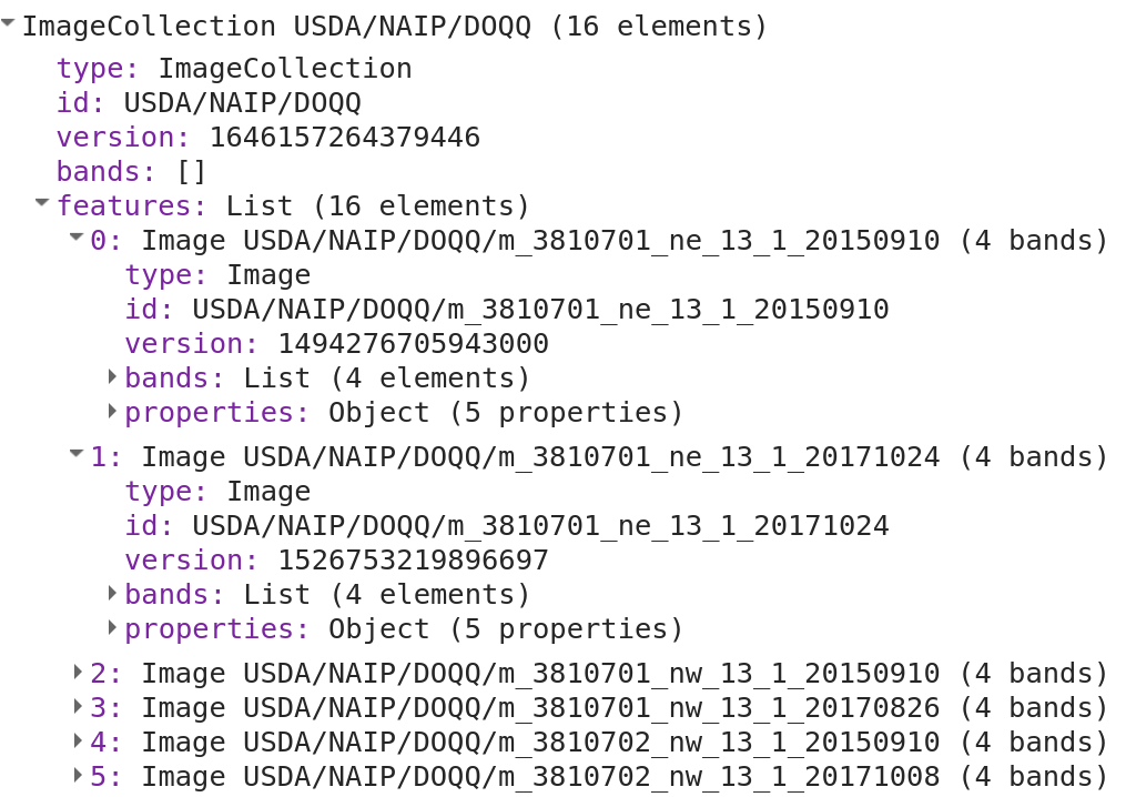
The print statement shows us that imagery is available for both 2015 and 2017, yet it is difficult to determine the extent of coverage present without visualizing the data. For now, we will add both collections to the map to see what the image availability looks like. Add the following code to your existing script.

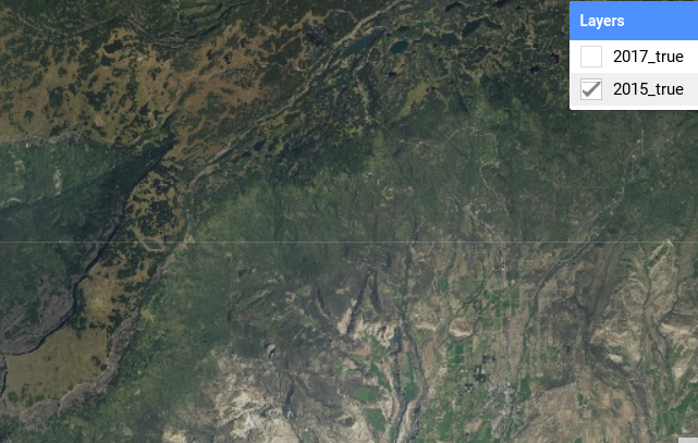
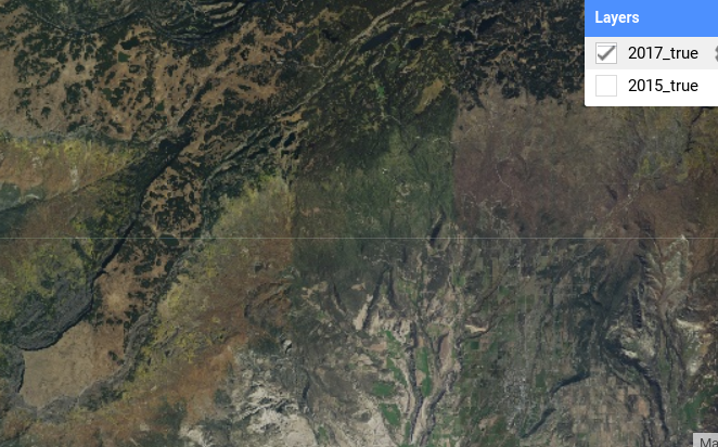
Compared to the 2015 imagery (Fig. A3.7.3), the 2017 imagery (Fig. A3.7.4) has been captured later in the season and we can start to see some yellow in the aspen. A challenge with this image is that there were some distinct time lags between neighboring flight paths during the initial image collection. Notice the vertical band of green in the 2017 image. While it is usually best practice to use images that closely match the time that you will be in the field, in this case the consistency of the 2015 imagery outweighs those temporal concerns.

We will also add a false color image to the 2015 data because this band combination visualization is very helpful for distinguishing between deciduous and coniferous forests. We do this by adding the naip2015 object with a different set of visualization parameters to the map. Add the following code to your existing script.

Section 1.3. Aspen Exclosures

In our hypothetical study, let us imagine land managers have established some aspen exclosures on the southern extent of the Grand Mesa. Let us also say that the land managers did not have specific shapefiles of the exclosures but did have GPS locations of the four corners. We will use these data to add the exclosures to the map by creating a geometry feature within our script. In this case we are creating an ee.Geometry.MultiPolygon feature. Add the following code to your existing script. If your roi object does not encompass the exclosures, edit its bounds or redraw it.

The structure of the ee.Geometry.MultiPolygon feature is a bit complex, but it is effectively a set of nested lists. There are three tiers of lists present:

• Tier 1: A single list that holds all the data. The ee.Geometry.MultiPolygon function requires the input to be a list.
• Tier 2: A list for each polygon, containing a unique set of coordinates.
• Tier 3: A list for each x,y coordinate pair. Each polygon is composed of a series of x,y points with a point that overlaps exactly with the first coordinate pair. This last coordinate pair is the same as the first and is essential to completing the feature.

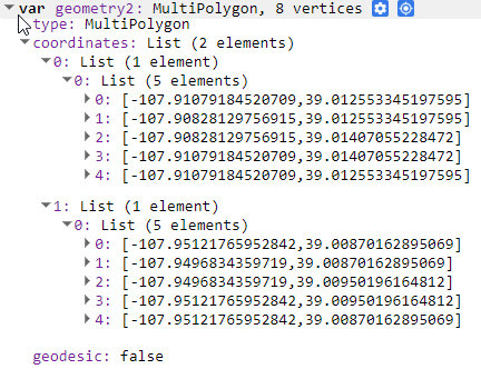
If you are trying to make a geometry feature and are having trouble, you can always create one with the draw shape tool and look at the values in a print statement as a template (Fig. A3.7.5).

Section 1.4. Determining Similar Areas for Sampling

Now that we have our aspen exclosures loaded, we are going to bring in some additional layers to help quantify the landscape characteristics of the exclosures. We will use those values to find similar areas nearby to use as sampling sites outside of the exclosures. By keeping the environmental conditions similar, we can make stronger statements about the comparative effects of herbivory on aspen stands.

We will use three datasets to describe the conditions within the sampled areas:

1. NED: Select areas in a similar elevation range. Elevation is correlated with many environmental conditions, so we are using it as a proxy for features such as temperature, precipitation, and solar radiation.
2. NAIP: Calculate an NDVI index to get a measure of vegetation productivity.
3. NLCD: Select the deciduous forest class as a way to limit the location of sampling sites.

Section 1.5. Loading in the Data

First, we will call the NED by its unique ID. We can gather these details by searching for the feature and reading through the metadata. Add the following code to your existing script.

We already have NAIP imagery loaded but we need to convert it to an image and calculate NDVI. We have already filtered our NAIP imagery to a single year, so there is only one image per area. We could apply a reducer to convert the ImageCollection to an image, but a reducer is not necessary for a single layer. A more logical option for this is to apply the mosaic function to convert the ImageCollection to an image. Add the following code to your existing script.

The last dataset we are bringing in is the NLCD. Add the following code to your existing script.

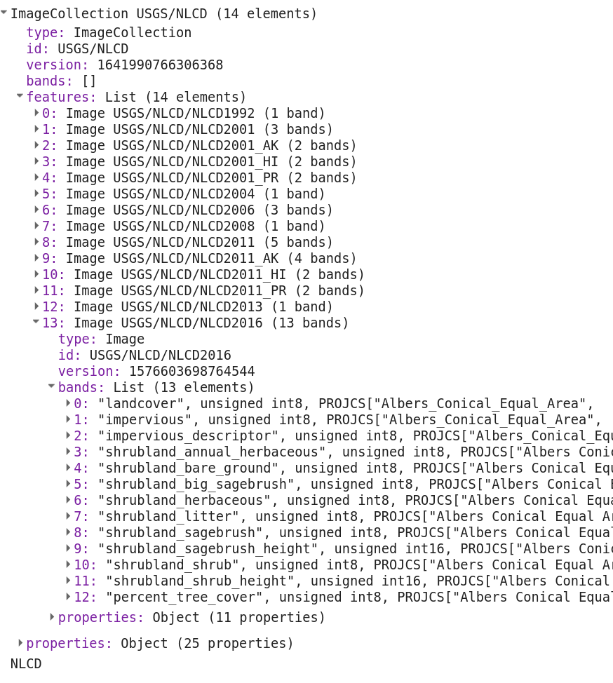
From the print statement (Fig. A3.7.6), we can see that some of the images have a band called 'landcover'. Rather than trying to pull it out from the feature collection, we will call the 2016 NLCD image directly by its unique ID and select the 'landcover' band.

Question 1. Investigate the other available years in the NLCD collection. What parts of the study area have land cover classes that change? What might be driving that change?

Section 1.6. Generating Random Points

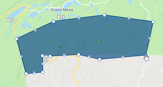
With our three datasets loaded we can now generate a series of potential survey sites. We will do this by generating random points within a given area (Fig. A3.7.7). We want these sites to be accessible, near the two exclosures, and within the public land boundary. We will create another geometry feature that we will use to contain the randomly generated points. Hover over the Geometry imports box and click +new layer. Be sure to name this second geometry feature sampleArea.

With the geometry feature in place, we can create points using the randomPoints function. Add the following code to your existing script.

Here, we are using a dictionary to define the parameters of the function. The region parameter is the area in which the points are created. In our case, we are going to set this to sampleArea polygon. The points parameter specifies the total number of points to generate. The seed parameter is used to indicate specific random values. Think of this as a unique ID for a set of random values. The seed number (1234 in this example) refers to an existing random list of values. Setting the seed is very helpful because you are still using random values, but the code will place the points in the same locations every time until the seed is changed.

Section 1.7. Extracting Values to Points

To associate the landscape characteristics with the point locations, we are going to call the ee.Image.sampleRegions function. This function requires a single image. Rather than calling three times on our three unique images (elevation, NDVI, and NLCD), we are going to add all those images together to create a multiband image so we can call this function a single time. Add the following code to your existing script.

With the multiband image set, we will call the sampleRegions function. Add the following code to your existing script.

Within this function, the collection parameter is set to the feature collection where the extracted values will be added. In this example it is a point dataset. The scale parameter refers to the spatial resolution (pixel size) of the data. The geometries parameter indicates whether or not you want to maintain the x,y coordinate pairs for each element in the collection. The default is false, but we set it to true here because we eventually want to show these points on the map, as they will represent suitable sampling site locations.

Segue on Scale 

The idea of scale is very important in remote sensing, but you will often encounter multiple definitions of it. Map scale, the relationship between a measured distance on a map and the actual distance on the landscape, is the most common in remote sensing. The image extent can also be referred to as the scale of the image or the spatial scale. Confusing, right?

In the case of the scale argument in the function above, it is referring to yet another definition of that word—the pixel size of the image. In our example, the multiband image has two bands with a pixel size of 30 m, and one with a pixel size of 1 m. It is best practice to use the largest pixel size when working with data having different spatial resolutions. Here, this means you are upscaling the 1 m image to 30 m. This means a potential loss of precision in your data. However, you can be confident that the number in that upscaled cell is representative of the mean value across all the cells. If you go in the opposite direction and downscale an image, you effectively make up the data to fill the gap. Because NAIP imagery has a 1 m pixel size, it contains 30 x 30 more pixels than a single 30 m pixel. Take a look at the examples below to help visualize these processes.

Upscaling takes the available data and finds the mean value.

| 3 | 7 | 8 |

| 4 | 2 | 2 |

| 1 | 3 | 2 |

Question 2. Calculate the mean for the matrix above. How would this value change your understanding of the pixel? Is it still representative of the overall “story” the data is telling, or would a different reducer (i.e., median) be more appropriate?

Downscaling takes a single value and places the value for all locations in the grid.

| 7 | 7 | 7 |

| 7 | 7 | 7 |

| 7 | 7 | 7 |

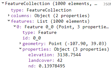
From our print statement (Fig. A3.7.8) we can see that each of our 1000 point locations have three properties: elevation, land cover, and NDVI. We want to use these values to filter out sites that do not match the conditions of the exclosures. The land cover data are categorical, so it is easy to filter. We know from the metadata on NLCD that the land cover class for deciduous forest is a single value (41).

We will use the filter function to select all sites that are within aspen forests. Add the following code to your existing script.

From the print statement, we can see this reduces the total number of potential sites (1000) by about 25%, depending on your study area shape. However, to get down to roughly 10 potential new monitoring sites, there is still a lot of trimming to do.

Filtering based on elevation and NDVI is a bit trickier because both of these variables are continuous data. You want to find sites that have similar values to those in the exclosures, but they do not need to be exactly the same. For this example, we will say that if a value is within ±10% of the mean value found within the exclosure, we will group it as similar. There are a couple of things that need to be calculated before we can filter our potential sampling sites:

1. Mean values within exclosures.
2. 10% above and below the mean.

Question 3. The above use of ±10% is somewhat arbitrary. How might the range change given the inclusion of additional exclosures in our study area? What other methods could be used to generate this range?

We will work with the NDVI image first and then apply this process to the elevation dataset.

• Step 1: To find the mean value, we are going to apply a mean reducer over the area that is inside of the exclosure. Add the following code to your existing script.

The reduceRegion function takes in an image and returns a dictionary where the key is the name of the band, and the value is the output of the reducer.

• Step 2: Determine the acceptable variability around the mean.

We are relying on simple mathematical functions to find the ±10% values. Add the following code to your existing script.

The first step in this process is all about understanding data types. The ndvi1 object is a dictionary so we call the get function to pull a value based on a known key. We then convert that value to an ee.Number type object so we can apply the math functions. Our output is a list with the minimum and maximum values (±10% of the mean NDVI values).

Section 1.8. Create Your Own Function

We now have our range for NDVI, but we also need to apply the same process to elevation. In this case we are only applying this process twice, but it seems like a useful chunk of code that might be handy down the road. Rather than just copying and pasting the code again and again, we are going to create a function with flexible parameters so we can apply this useful bit of code efficiently.

A function has the following requirements: parameters, statements, and a return value. Here is an example of the structure of a function from the official Earth Engine documentation. The following pseudocode demonstrates the syntax and structure of a function in JavaScript. Do not add this code to your script.

If we apply this structure to our goal of reducing the elevation by area (like we did for NDVI with the code we created above), we would need to consider the following:

• Parameters : an image, a geometry object, and pixelSize.
• Statements: reduceRegion function.
• A return value: output of the reduceRegion function.

When using functions, it is important to use informative names within your parameters that give some indication of the data type that is required. If we want our function to be reproducible, we can provide some more information as a longer comment when we define the function. Add the following code to your existing script.

Let’s check our function definition by verifying that it gives the same answer for the NDVI range as when we did it step by step:

This is a very clean method for coding when you need to apply a process multiple times.The function has been defined and now we can call it on the elevation dataset. Add the following code to your existing script.

 We will define a second function to determine ±10% around a mean value.

• Parameters: an image, band name, proportion.
• Statements: multiple steps.
• A return value: list.

Add the following code to your existing script.

We will call the effectiveRange function on the output of the reduceRegionFunction function. Add the following code to your existing script.

Now that we have an effective range for both our NDVI and elevation values, we can apply an additional set of filters to thin the list of potential sample sites. We can do this by chaining multiple ee.Filter calls together. Add the following code to your existing script.

Depending on how you have drawn your study area, this filtering process should reduce the 1000 original sites by about 90%. From the ~100 remaining sites, we can manually select 10 either by something we already know about the landscape features of our study area, or by using a more restrictive range in our function (e.g., ±5%). This approach to site selection can be a good first step in ensuring you are sampling similar conditions in the field.

Code Checkpoint A37a. The book’s repository contains a script that shows what your code should look like at this point.

Section 2. Generating Your Own Training Dataset

As you have been examining this landscape, you may have noticed some misclassifications within the NLCD land cover layer (e.g., forests in non-forested areas). Some misclassifications are expected in any land cover dataset. While the NLCD is trained to produce classifications of specific land cover assemblages across the United States, the aspen forest class that we are examining is included within a much larger grouping (“Deciduous forest”). Also, the particular NLCD image we selected shows land cover as it was detected in 2011. While forests are fairly stable over time, we can expect that some level of change has occurred. This might get you thinking about the possibility of generating your own aspen land cover product based on a remote sensing model for this specific region. There is a lot that goes into this process that we are not going to cover here. However, we are going to take the first step, which is generating our own presence/absence training dataset.

Section 2.1. Ocular Sampling

Generating your own training data relies on the assumption that you can confidently identify your species of interest using high-resolution imagery. We are using NAIP for this process because it is freely available and has a known collection date, allowing us to mark areas of aspen forest as “presence” and areas without aspens as “absence.” These data could then be used later to train a model of aspen occurrence on the landscape.

Section 2.2. Adding Presence and Absence Points

First, we will need to create specific layers that will hold our new sampling points. Adding in presence and absence layers is a straightforward process accomplished by manually creating and placing geometry features on representative locations on the map. Hover over the Geometry imports box and click +new layer (Fig. A3.7.9). A geometry feature named “geometry” will be added. Select the gear icon next to geometry and a pop-up will open. Change the Import as type to FeatureCollection, then press the +Add property button. Fill in the Properties values with “presence” and “1” and press OK to save your feature.

Change the feature collection name to presence and select a color you enjoy. Repeat this process to create an absence feature collection where the added property values are presence and “0". We will use the binary value in the presence column of both datasets to define what that location is referring to: 1=Yes, this is aspen; 0=No, this is not aspen.

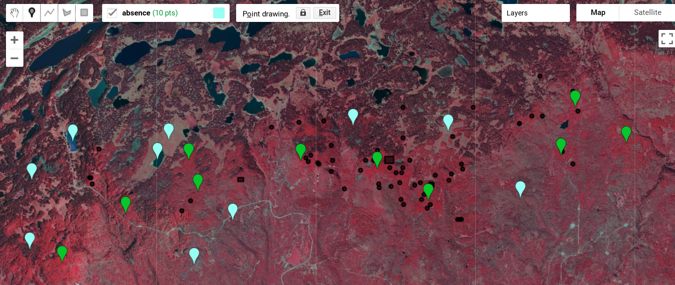
Once the feature collections are created, we select the specific feature collection (presence or absence) and use the marker tool to drop points on the imagery. The sampling methodology you use will depend on your study. In this example, green presence points represent aspen forest, and blue points are not aspen (absence).

Use the 2015 false-color imagery in combination with the NDVI or NLCD to distinguish aspen from other land cover types. Aspen stands are brighter red than most other vegetation types and tend to have a more complex texture than herbaceous vegetation in the imagery. Drop some points in what you perceive to be aspen forest (Fig. A3.7.10).

Feel free to sample as many locations as you would like. Again, the quality of this data will depend on your ability to differentiate the multiple land cover classes present.

Section 2.3. Exporting Points

Currently our point locations are stored in two different features classes. We will merge these features into one feature class before exporting the data. We can merge the layers straightforwardly because they share the same data type (point geometry feature) and the same attribute data (“presence” with a numeric data value). Add the following code to your existing script.

Now that the sampling features classes are merged, we will export the features to our Google Drive. When you run the code below, the Tasks tab in the upper right-hand panel will light up. Earth Engine does not run tasks without you directing it to execute the task from the Tasks tab. Add the following code to your existing script and run it to export your completed dataset.

Code Checkpoint A37b. The book’s repository contains a script that shows what your code should look like at this point.

Synthesis

Assignment 1. Compare samples of NDVI ranges for aspen presence versus absence. Are the ranges significantly different? Create samples using the code presented here but for a coniferous tree of your choice. How different are these values from the values of deciduous forest?

Conclusion

In this module, we identified aspen locations with similar environmental characteristics and generated our own sampling data from those locations. Both processes are simple in concept but can be somewhat complex to implement without access to all your data in a single place. In both cases, we are generating value-added products that are informed by remote sensing but are not inherently remote sensing processes. This ability to be creative regarding how you use remotely sensed data is part of the beauty of the Earth Engine platform.

Feedback

To review this chapter and make suggestions or note any problems, please go now to bit.ly/EEFA-review. You can find summary statistics from past reviews at bit.ly/EEFA-reviews-stats.

References

Cloud-Based Remote Sensing with Google Earth Engine. (n.d.). CLOUD-BASED REMOTE SENSING WITH GOOGLE EARTH ENGINE. https://www.eefabook.org/

Cloud-Based Remote Sensing with Google Earth Engine. (2024). In Springer eBooks. https://doi.org/10.1007/978-3-031-26588-4

Halofsky J, Ripple W (2008) Linkages between wolf presence and aspen recruitment in the Gallatin elk winter range of southwestern Montana, USA. Forestry 81:195–207. https://doi.org/10.1093/forestry/cpm044