Aquatic and Hydrological Applications

Defining Seasonality First Date of No Snow

Cloud-Based Remote Sensing with Google Earth Engine

Fundamentals and Applications

Part A2: Aquatic and Hydrological Applications

Earth Engine’s global scope and long time series allow analysts to understand the water cycle in new and unique ways. These include surface water in the form of floods and river characteristics, long-term issues of water balance, and the detection of subsurface ground water.

Chapter A2.6: Defining Seasonality: First Date of No Snow

Authors

Amanda Armstrong, Morgan Tassone, Justin Braaten

Overview

The purpose of this chapter is to demonstrate how to produce annual maps representing the first day within a year on which a given pixel reaches 0% snow cover. It also provides suggestions for summarizing and visualizing the results over time and space.

Learning Outcomes

Generating and using a date band in image compositing.
Applying temporal filtering to an ImageCollection.
Identifying patterns of seasonal snowmelt.

Helps if you know how to:

Import images and image collections, filter, and visualize (Part F1).
Perform basic image analysis: select bands, compute indices, create masks (Part F2).
Work with time-series data in Earth Engine (Part F4).
Fit linear and nonlinear functions with regression in an ImageCollection time series (Chap. F4.6).

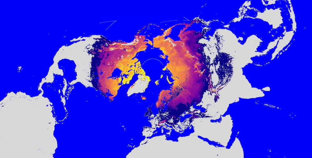
Fig. A2.6.1 Arctic polar stereographic projection showing the pattern of snowmelt timing in the Northern Hemisphere. The image shows the first day in 2018 on which each pixel no longer contained snow, as detected by the Moderate Resolution Imaging Spectroradiometer (MODIS) Snow Cover Daily Global product. The color grades from purple (earlier) to yellow (later).

Github Code link for all tutorials

This code base is collection of codes that are freely available from different authors for google earth engine.

Github Source

Introduction to Theory

The timing of annual seasonal snowmelt (Fig. A2.6.1) and any potential change in that timing have broad ecological implications and thus impact human livelihoods, particularly in and around high-latitude and mountainous systems. The annual melting of accumulated winter snowfall, one of the most important phases of the hydrologic cycle within these regions, provides the dominant source of water for streamflow and groundwater recharge for approximately one sixth of the global population (Musselman et al. 2017, Barnhart et al. 2016, Bengtsson 1976). The timing of snowmelt in the Arctic and Antarctic influences the length of the growing season, and consistent snow cover throughout the winter insulates vegetation from harsh temperatures and wind (Duchesne et al. 2012, Kudo et al. 1999). In mountainous regions, such as the Himalayas, snowmelt is a major source of freshwater downstream (Barnhart et al. 2016) and is essential in recharging groundwater.

This seasonal water resource is one of the fastest-changing hydrologic systems under Earth’s warming climate, and these changes will broadly impact regional economies and ecosystem functioning, and increase the potential for flood hazards (Musselman et al. 2017, IPCC 2007, Beniston 2012, Allan and Casillo 2007, Barnett and Lettenmaier 2005). An analysis focusing on the Yamal Peninsula in the northwestern Siberian tundra found that the timing of snowmelt (calculated using the methods outlined here) was an important predictor of differences in ecosystem functioning across the landscape (Tassone et al., in prep).

The anticipated warmer temperatures will alter the type and onset of precipitation. Multiple regions, including the Rocky Mountains of North America, have already measured a reduction in snowpack volume, and warmer temperatures have shifted precipitation from snowfall to rain, causing snowmelt to occur earlier (Barnhart et al. 2016, Clow 2010, Harpold et al. 2012).

This tutorial demonstrates how to calculate the first day of no snow annually at the pixel level, providing the user with the ability to track the seasonal and interannual variability in the timing of snowmelt toward a better understanding of how the hydrological cycles of higher-latitude and mountainous regions are responding to climate change.

Practicum

Section 1. Identifying the First Day of 0% Snow Cover

This section covers building an ImageCollection where each image is a mosaic of pixels that describe the first day in a given year that 0% snow cover was recorded. Snow cover is defined by the MODIS Normalized Difference Snow Index (NDSI) Snow Cover Daily Global product. The general workflow is as follows.

Define the date range to consider for analysis.
Define a function that adds date information as bands to snow cover images.
Define an analysis mask.
For each year:

Filter the ImageCollection to observations from the given year.
Add date bands to the filtered images.
Identify the first day of the year without any snow per pixel.
Apply an analysis mask to the image mosaic.
Summarize the findings with a series of visualizations.

Section 1.1. Define the Date Range

First, we specify the day of year (DOY) on which to start the search for the first day with 0% snow cover. For applications in the Northern Hemisphere, you will likely want to start with January 1 (DOY 1). However, if you are studying snowmelt timing in the Southern Hemisphere (e.g., the Andes), where snowmelt can occur on dates on either side of January 1, it is more appropriate to start the year on July 1 (DOY 183), for instance. In this calculation, a year is defined as the 365 days beginning from the specified startDoy.

var startDoy=1;

Then, we define the years to start and end tracking snow-cover fraction. All years in the range will be included in the analysis.

var startYear=2000;
var endYear=2019;

Section 1.2. Define the the Date Bands

Next, we will define a function to add several date bands to the images; the added bands will be used in a future step. Each image has a metadata timestamp property, but since we will be creating annual image mosaics composed of pixels from many different images, the date needs to be encoded per pixel as a value in an image band so that it is retained in the final mosaics. The function encodes:

Calendar DOY (calDoy): enumerated DOY from January 1.
Relative DOY (relDoy): enumerated DOY from a given startDoy.
Milliseconds elapsed since the Unix epoch (millis).
Year (year): Note that the year is tied to the startDoy. For example, if the startDoy is set at 183, the analysis will cross into the next calendar year, and the year given to all pixels will be the earlier year, even if a particular image was collected on or after January 1 of the subsequent year.

Additionally, two global variables are initialized (startDate and startYear) that will be redefined iteratively in a subsequent step.

var startDate;
var startYear;

function addDateBands(img){
// Get image date.
var date=img.date();
// Get calendar day-of-year.
var calDoy=date.getRelative('day', 'year');
// Get relative day-of-year; enumerate from user-defined startDoy.
var relDoy=date.difference(startDate, 'day');
// Get the date as milliseconds from Unix epoch.
var millis=date.millis();
// Add all of the above date info as bands to the snow fraction image.
var dateBands=ee.Image.constant([calDoy, relDoy, millis,
startYear
])
.rename(['calDoy', 'relDoy', 'millis', 'year']);
// Cast bands to correct data type before returning the image.
return img.addBands(dateBands)
.cast({
'calDoy': 'int',
'relDoy': 'int',
'millis': 'long',
'year': 'int'
})
.set('millis', millis);
}

Section 1.3. Define an Analysis Mask

Here is the opportunity to define a mask for your analysis. This mask can be used to constrain the analysis to certain latitudes, land cover types, geometries, etc. In this case, we will (1) mask out water so that the analysis is confined to pixels over landforms only, (2) mask out pixels that have very few days of snow cover, and (3) mask out pixels that are snow covered for a good deal of the year (e.g., glaciers).

Import the MODIS Land/Water Mask dataset, select the 'water_mask' band, and set all land pixels to value 1.

var waterMask=ee.Image('MODIS/MOD44W/MOD44W_005_2000_02_24')
.select('water_mask')
.not();

Import the MODIS Snow Cover Daily Global 500 m product and select the 'NDSI_Snow_Cover' band.

var completeCol=ee.ImageCollection('MODIS/006/MOD10A1')
.select('NDSI_Snow_Cover');

Mask pixels based on the frequency of snow cover.

// Pixels must have been 10% snow covered for at least 2 weeks in 2018.
var snowCoverEphem=completeCol.filterDate('2018-01-01',
'2019-01-01')
.map(function(img){
return img.gte(10);
})
.sum()
.gte(14);

// Pixels must not be 10% snow covered more than 124 days in 2018.
var snowCoverConst=completeCol.filterDate('2018-01-01',
'2019-01-01')
.map(function(img){
return img.gte(10);
})
.sum()
.lte(124);

Combine the water mask and the snow cover frequency masks.

var analysisMask=waterMask.multiply(snowCoverEphem).multiply(
snowCoverConst);

Section 1.4. Identify the First Day of the Year Without Snow Per Pixel, Per Year

Make a list of the years to process. The input variables were defined in Sect. 1.1.

var years=ee.List.sequence(startYear, endYear);

Map the following function over the list of years. For each year, identify the first day with 0% snow cover.

Define the start and end dates to filter the dataset for the given year.
Filter the ImageCollection by the date range.
Add the date bands to each image in the filtered collection.
Sort the filtered collection by date. (Note: To determine the first day with snow accumulation in the fall, reverse-sort the filtered collection.)
Make a mosaic using the min reducer to select the pixel with 0 (minimum) snow cover. Since the collection is sorted by date, the first image with 0 snow cover is selected. This operation is conducted per-pixel to build the complete image mosaic.
Apply the analysis mask to the resulting mosaic.

An ee.List of images is returned.

var annualList=years.map(function(year){
// Set the global startYear variable as the year being worked on so that
// it will be accessible to the addDateBands mapped to the collection below.
startYear=year;
// Get the first day-of-year for this year as an ee.Date object.
var firstDoy=ee.Date.fromYMD(year, 1, 1);
// Advance from the firstDoy to the user-defined startDay; subtract 1 since
// firstDoy is already 1. Set the result as the global startDate variable so
// that it is accessible to the addDateBands mapped to the collection below.
startDate=firstDoy.advance(startDoy - 1, 'day');
// Get endDate for this year by advancing 1 year from startDate.
// Need to advance an extra day because end date of filterDate() function
// is exclusive.
var endDate=startDate.advance(1, 'year').advance(1,
'day');
// Filter the complete collection by the start and end dates just defined.
var yearCol=completeCol.filterDate(startDate, endDate);
// Construct an image where pixels represent the first day within the date
// range that the lowest snow fraction is observed.
var noSnowImg=yearCol
// Add date bands to all images in this particular collection.
.map(addDateBands)
// Sort the images by ascending time to identify the first day without
// snow. Alternatively, you can use .sort('millis', false) to
// reverse sort (find first day of snow in the fall).
.sort('millis')
// Make a mosaic composed of pixels from images that represent the
// observation with the minimum percent snow cover (defined by the
// NDSI_Snow_Cover band); include all associated bands for the selected
// image.
.reduce(ee.Reducer.min(5))
// Rename the bands - band names were altered by previous operation.
.rename(['snowCover', 'calDoy', 'relDoy', 'millis',
'year'
])
// Apply the mask.
.updateMask(analysisMask)
// Set the year as a property for filtering by later.
.set('year', year);

// Mask by minimum snow fraction - only include pixels that reach 0
// percent cover. Return the resulting image.
return noSnowImg.updateMask(noSnowImg.select('snowCover')
.eq(0));
});

Convert the ee.List of images to an ImageCollection.

var annualCol=ee.ImageCollection.fromImages(annualList);

Code Checkpoint A26a. The book’s repository contains a script that shows what your code should look like at this point.

Section 2. Data Summary and Visualization

The following is a series of examples for how to display and explore the “first DOY with no snow” dataset you just generated.

These examples refer to the calendar date (calDoy band) when displaying and incorporating date information in calculations. If you are using a date range that begins on any day other than January 1 (DOY 1) you may want to replace calDoy with relDoy in all cases below.
Results may appear different as you zoom in and out of the Map because of tile aggregation, which is described in the Earth Engine documentation. It is best to view Map data interactively with a relatively high zoom level. Additionally, for any analysis where a function provides a scale parameter (e.g., region reduction, exporting results), it is best to define it with the native resolution of the dataset (500 m).
MODIS cloud masking can influence results. If there are a number of sequentially masked image pixel observations (e.g., clouds, poor quality), the actual date of the first observation with 0% snow cover may be earlier than identified in the image time series. Regional patterns may be less influenced by this bias than local results. For local results, please inspect image masks to understand their influence on the dates near snowmelt timing.

Section 2.1. Single-Year Map

Filter a single year from the collection (2018 in the example below) and display the image to the Map to see spatial patterns of snowmelt timing. Setting the min and max parameters of the visArgs variable to a narrow range around expected snowmelt timing is important for getting a good color stretch.

// Define a year to visualize.
var thisYear=2018;

// Define visualization arguments.
var visArgs={
bands: ['calDoy'],
min: 150,
max: 200,
palette: [
'0D0887', '5B02A3', '9A179B', 'CB4678', 'EB7852',
'FBB32F', 'F0F921'
]
};

// Subset the year of interest.
var firstDayNoSnowYear=annualCol.filter(ee.Filter.eq('year',
thisYear)).first();

// Display it on the map.
Map.setCenter(-95.78, 59.451, 5);
Map.addLayer(firstDayNoSnowYear, visArgs,
'First day of no snow, 2018');

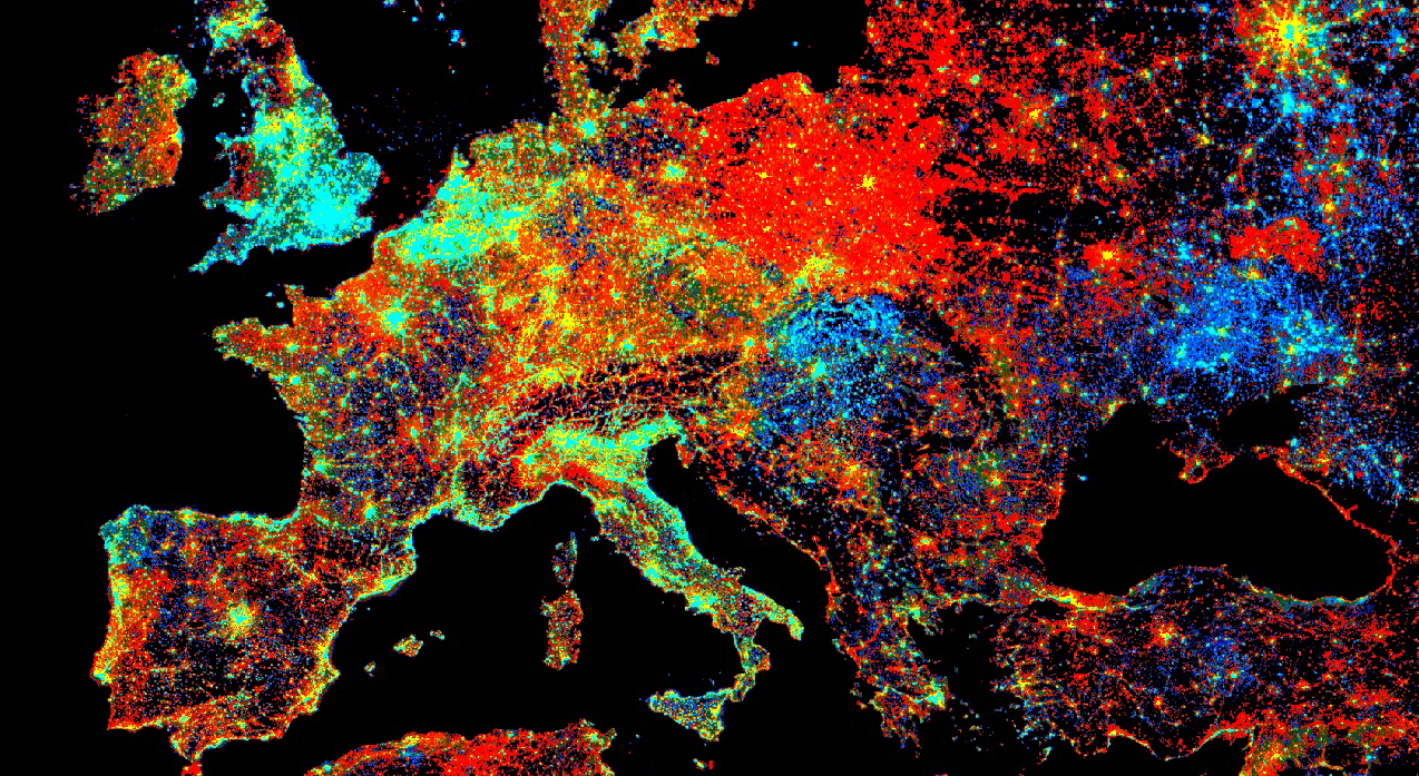
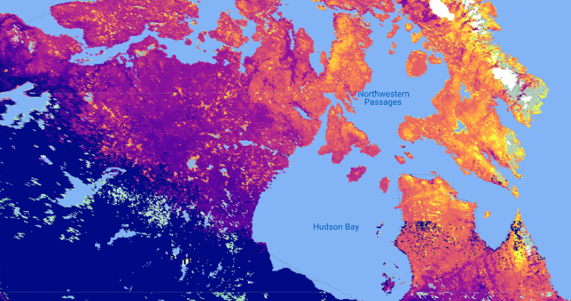
Running this code produces something similar to Fig. A2.6.2. The color represents the DOY when 0% snow cover was first observed per pixel (blue is earlier, yellow is later).

One can notice a number of interesting patterns. Frozen lakes have been shown to decrease air temperatures in adjacent pixels, resulting in delayed snowmelt (Rouse et al. 1997, Salomonson and Appel 2004, Wang and Derksen 2007). Additionally, the protected estuaries of the Northwest Passages have earlier dates of no snow compared to the landscapes exposed to the currents and winds of the Northern Atlantic. Latitude, elevation, and proximity to ocean currents are the strongest determinants in this region.

Note that pixels representing glaciers that did not get removed by the analysis mask can produce anomalies in the data. Since glaciers are generally snow covered, the DOY with the least snow cover according to the MODIS Snow Cover Daily Global product is presented in the Map. In Fig. A2.6.2, this is evident in the abrupt transition within alpine areas of Baffin Island (white pixels represent glaciers in this case).

Fig. A2.6.2 Thematic map representing the first DOY with 0% snow cover. Color grades from blue to yellow as the DOY increases.

Section 2.2. Year-to-Year Difference Map

Compare year-to-year difference in snowmelt timing by selecting two years of interest from the collection and subtracting them. Here, we’re calculating the difference in snowmelt timing between 2005 and 2015.

// Define the years to difference.
var firstYear=2005;
var secondYear=2015;

// Calculate difference image.
var firstImg=annualCol.filter(ee.Filter.eq('year', firstYear))
.first().select('calDoy');
var secondImg=annualCol.filter(ee.Filter.eq('year', secondYear))
.first().select('calDoy');
var dif=secondImg.subtract(firstImg);

// Define visualization arguments.
var visArgs={
min: -15,
max: 15,
palette: ['b2182b', 'ef8a62', 'fddbc7', 'f7f7f7', 'd1e5f0',
'67a9cf', '2166ac'
]
};

// Display it on the map.
Map.setCenter(95.427, 29.552, 8);
Map.addLayer(dif, visArgs, '2015-2005 first day no snow dif');

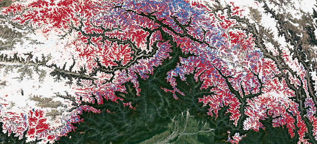
Running this code produces something similar to Fig. A2.6.3. The color represents the difference, in each pixel, between the 2005 and 2015 DOY when 0% snow cover was first observed. Red represents a negative change (an earlier no-snow date in 2015), blue represents a positive change (a later no-snow date in 2015), and white represents a negligible or no change in the no-snow dates for 2005 and 2015.

Fig. A2.6.3 Year-to-year (2005–2015) difference map of the Himalayas on the Nepal–China border. Color grades from red to blue, with red indicating an earlier date of no snow in 2015 and blue indicating a later date of no snow in 2015. White areas indicate little or no change.

Section 2.3. Trend Analysis Mapping

It is also possible to identify trends in the shifting first DOY with no snow by calculating the slope through a pixel’s time-series points. Here, the slope for each pixel is calculated with year as the x variable and the first DOY with no snow as the y variable.

// Calculate slope image.
var slope=annualCol.sort('year').select(['year', 'calDoy'])
.reduce(ee.Reducer.linearFit()).select('scale');

// Define visualization arguments.
var visArgs={
min: -1,
max: 1,
palette: ['b2182b', 'ef8a62', 'fddbc7', 'f7f7f7',
'd1e5f0', '67a9cf', '2166ac'
]
};

// Display it on the map.
Map.setCenter(11.25, 59.88, 6);
Map.addLayer(slope, visArgs, '2000-2019 first day no snow slope');

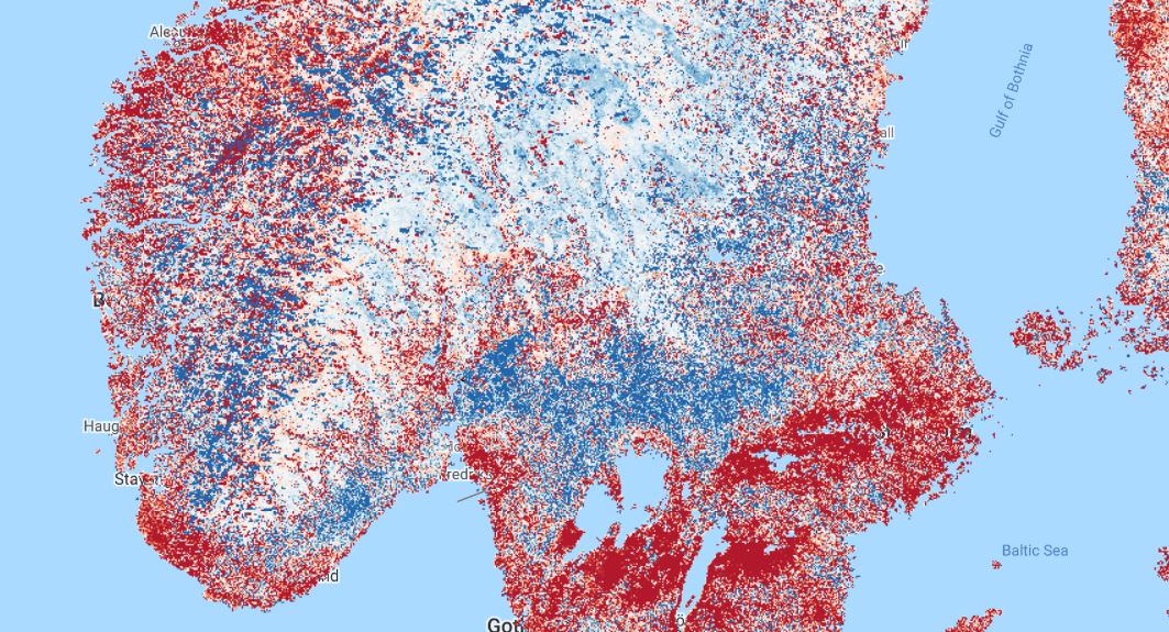
The result is a map (Fig. A2.6.4) where red represents a negative slope (progressively earlier first DOY with no snow), white represents a slope of 0, and blue represents a positive slope (progressively later first DOY with no snow). In southern Norway and Sweden, the trend in the first DOY with no snow between 2002 and 2019 appears to be influenced by various factors. Coastal areas exhibit progressively earlier first DOY of no snow than inland areas; however, high variability in slopes can be observed around fjords and in mountainous regions. This map reveals the complexity of seasonal snow dynamics in these areas.

Note that goodness-of-fit calculations are not measured here, nor is significance considered. While a slope can indicate regional trends, more local trends should be investigated using a time-series chart (see the next section). Interannual variability can be influenced by masked pixels, as described above.

Fig. A2.6.4 Map representing the slope of the first DOY with no snow cover between 2000 and 2019. The slope represents the overall trend. Color grades from red (negative slope) to blue (positive slope). White indicates areas of little to no change.

Section 2.4. Time-Series Chart

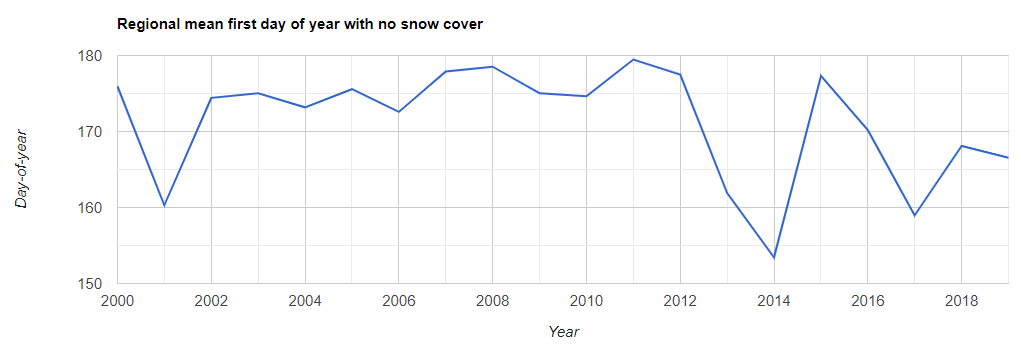
To visually understand the temporal patterns of the first DOY with no snow through time, we can display our results in a time-series chart. In this case, we’ve defined a circle with a radius of 500 m around a point of interest and calculated the annual mean first DOY with no snow for pixels within that circle.

// Define an AOI.
var aoi=ee.Geometry.Point(-94.242, 65.79).buffer(1e4);
Map.addLayer(aoi, null, 'Area of interest');

// Calculate annual mean DOY of AOI.
var annualAoiMean=annualCol.select('calDoy').map(function(img){
var summary=img.reduceRegion({
reducer: ee.Reducer.mean(),
geometry: aoi,
scale: 1e3,
bestEffort: true,
maxPixels: 1e14,
tileScale: 4,
});
return ee.Feature(null, summary).set('year', img.get(
'year'));
});

// Print chart to console.
var chart=ui.Chart.feature.byFeature(annualAoiMean, 'year',
'calDoy')
.setOptions({
title: 'Regional mean first day of year with no snow cover',
legend:{
position: 'none'
},
hAxis:{
title: 'Year',
format: '####'
},
vAxis:{
title: 'Day-of-year'
}
});
print(chart);

Code Checkpoint A26b. The book’s repository contains a script that shows what your code should look like at this point.

As is evident in the displayed results (Fig. A2.6.5), the first DOY with no snow was mostly stable from 2000 to 2012; following this, it has become more erratic.

Fig. A2.6.5 Annual mean first DOY with no snow time series for pixels within a small region of interest

Synthesis

Assignment 1. In Sect. 2.4, a time-series chart for a region of interest was generated. Suppose you wanted to compare several regions in the same chart; how would you change the code to achieve this? For instance, try plotting the first DOY of no snow at points (−69.271, 65.532) and (−104.484, 65.445) in the same chart. Some helpful functions include ee.Image.reduceRegions, ee.FeatureCollection.flatten, and ui.Chart.feature.groups.

Assignment 2. The objective of this chapter was to identify the first DOY of 0% snow cover. However, Sect. 1.4 provides a suggestion for altering the code to identify the last day of 0% snow cover. Can you modify the code to achieve this result?

Assignment 3. How could you determine regions that are often masked during the time of year when snowmelt occurs? (The results from such regions might not be reliable.) Hint: Think about how you can use the mask function on images, and investigate the 'NDSI_Snow_Cover_Class' and 'Snow_Albedo_Daily_Tile_Class' bands.

Conclusion

In this chapter, we provided a method to identify the annual, per-pixel, first DOY with no snow from MODIS snow cover image data. The result can be used to investigate patterns of seasonal snowmelt spatially and temporally. The method relied on adding a date band to each image in the collection, temporal sorting, and ImageCollection reduction. We demonstrated several different ways to analyze the results using map and chart interpretation, image differencing, and linear regression.

Feedback

To review this chapter and make suggestions or note any problems, please go now to bit.ly/EEFA-review. You can find summary statistics from past reviews at bit.ly/EEFA-reviews-stats.

References

Cloud-Based Remote Sensing with Google Earth Engine. (n.d.). CLOUD-BASED REMOTE SENSING WITH GOOGLE EARTH ENGINE. https://www.eefabook.org/

Cloud-Based Remote Sensing with Google Earth Engine. (2024). In Springer eBooks. https://doi.org/10.1007/978-3-031-26588-4

Allan JD, Castillo MM (2007) Stream Ecology: Structure and Function of Running Waters. Springer Nature

Barnhart TB, Molotch NP, Livneh B, et al (2016) Snowmelt rate dictates streamflow. Geophys Res Lett 43:8006–8016. https://doi.org/10.1002/2016GL069690

Bengtsson L (1976) Snowmelt estimated from energy budget studies. Nord Hydrol 7:3–18. https://doi.org/10.2166/nh.1976.0001

Beniston M (2012) Impacts of climatic change on water and associated economic activities in the Swiss Alps. J Hydrol 412–413:291–296. https://doi.org/10.1016/j.jhydrol.2010.06.046

Clow DW (2010) Changes in the timing of snowmelt and streamflow in Colorado: A response to recent warming. J Clim 23:2293–2306. https://doi.org/10.1175/2009JCLI2951.1

Duchesne L, Houle D, D’Orangeville L (2012) Influence of climate on seasonal patterns of stem increment of balsam fir in a boreal forest of Québec, Canada. Agric For Meteorol 162–163:108–114. https://doi.org/10.1016/j.agrformet.2012.04.016

Harpold A, Brooks P, Rajagopal S, et al (2012) Changes in snowpack accumulation and ablation in the intermountain west. Water Resour Res 48. https://doi.org/10.1029/2012WR011949

Kudo G, Nordenhäll U, Molau U (1999) Effects of snowmelt timing on leaf traits, leaf production, and shoot growth of alpine plants: Comparisons along a snowmelt gradient in northern Sweden. Ecoscience 6:439–450. https://doi.org/10.1080/11956860.1999.11682543

Musselman KN, Clark MP, Liu C, et al (2017) Slower snowmelt in a warmer world. Nat Clim Chang 7:214–219. https://doi.org/10.1038/nclimate3225

Rouse WR, Douglas MSV, Hecky RE, et al (1997) Effects of climate change on the freshwaters of arctic and subarctic North America. Hydrol Process 11:873–902. https://doi.org/10.1002/(SICI)1099-1085(19970630)11:8<873::AID-HYP510>3.0.CO;2-6

Salomonson VV, Appel I (2004) Estimating fractional snow cover from MODIS using the normalized difference snow index. Remote Sens Environ 89:351–360. https://doi.org/10.1016/j.rse.2003.10.016

Solomon S, Manning M, Marquis M, et al (2007) Climate change 2007- The Physical Science Basis: Working Group I Contribution to the Fourth Assessment Report of the IPCC. Cambridge University Press

Tassone M, Epstein HE (2020) Drivers of spatial and temporal variability in vegetation productivity on the Yamal Peninsula, Siberia, Russia. In: AGU Fall Meeting Abstracts. pp B084-04

Wang L, Derksen C, Brown R (2008) Detection of pan-Arctic terrestrial snowmelt from QuikSCAT, 2000-2005. Remote Sens Environ 112:3794–3805. https://doi.org/10.1016/j.rse.2008.05.017