Cloud-Based Remote Sensing with Google Earth Engine

Fundamentals and Applications

Part A2: Aquatic and Hydrological Applications
Earth Engine’s global scope and long time series allow analysts to understand the water cycle in new and unique ways. These include surface water in the form of floods and river characteristics, long-term issues of water balance, and the detection of subsurface ground water.
Chapter A2.5: Water Balance and Drought
Authors
Ate Poortinga, Quyen Nguyen, Nyein Soe Thwal, Andréa Puzzi Nicolau
Overview
In this chapter, you will learn simple water balance calculations using remote- sensing-derived products related to precipitation and evapotranspiration. You will work at the river basin scale and perform time-series analysis, while comparing the data series with remote sensing vegetation and drought indices using the Earth Engine platform. You will also overlay the various indices with a land cover map to estimate potential drought impacts throughout the region.
Learning Outcomes
- Understanding the basics of remote-sensing-derived precipitation and evapotranspiration products.
- Calculating monthly aggregate statistics.
- Performing time-series analysis.
- Calculating vegetation and drought indices.
Helps if you know how to:
- Import images and image collections, filter, and visualize (Part F1).
- Create a graph using ui.Chart (Chap. F1.3).
- Perform basic image analysis: select bands, compute indices, create masks (Part F2).
- Write a function and map it over an ImageCollection (Chap. F4.0).
- Summarize an ImageCollection with reducers (Chap. F4.0, Chap. F4.1).
- Aggregate data to build a time series (Chap. F4.2).
- Work with CHIRPS rainfall data (Chap. F4.2)
- Mask cloud, cloud shadow, snow/ice, and other undesired pixels (Chap. F4.3).
Github Code link for all tutorials
This code base is collection of codes that are freely available from different authors for google earth engine.
Introduction to Theory
Water is vital for sustaining human life, ensuring food security, generating power, and supporting industrial processes in river basins. Both terrestrial and aquatic ecosystems are dependent on water to provide valuable ecosystem services, not only for the current generation but also for generations in the future. Managing the complex flow paths of water to and from these different water-use sectors requires a quantitative understanding of hydrological processes. Quantitative insights are necessary to help manage water consumption more efficiently by means of retention, withdrawals, and land use change. Managers need background data to help them optimize water allocation to sectors without further depleting the natural capital in the basin.
Fig. A2.5.1 The key components of the hydrological cycle |
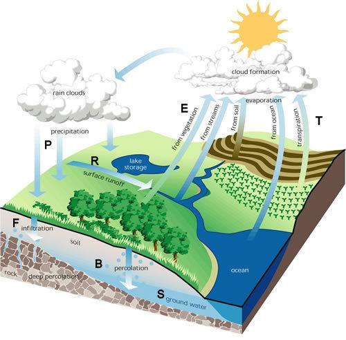
The water balance (Fig. A2.5.1) is the key concept in understanding the availability of water resources in a hydrological system. The water balance includes both input and extractions of water. In its simplest form, the water balance can be defined as Equation A2.5.1. Inputs to the hydrological system are defined by precipitation (P; rainfall and snow). Extractions for the system are from runoff (Q) and evapotranspiration (ET), with evapotranspiration denoting the sum of evaporation from the land surface plus transpiration from plants. Water balance changes in groundwater and soil storage are indicated by ΔS.
P =Q + ET + ΔS (A2.5.1)
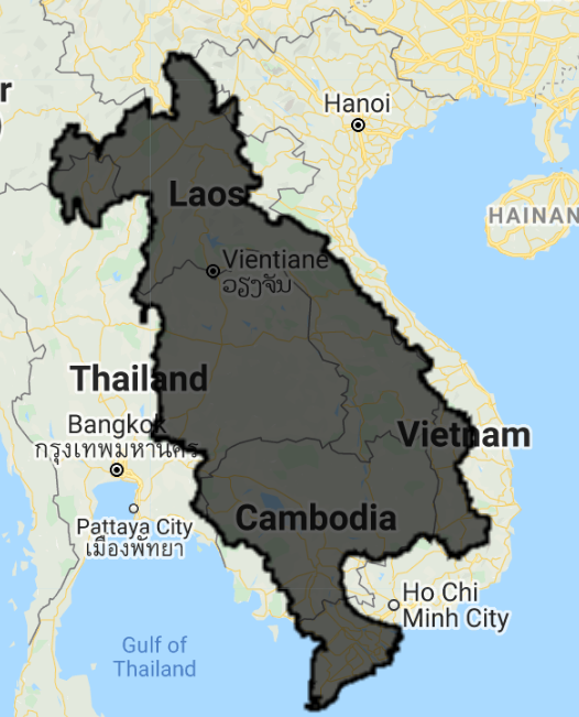
A hydrological system, also referred to as river basin or drainage basin, is any land area where precipitation collects and drains off into a common outlet. The hydrological processes between upstream and downstream are interconnected: For example, extractions of water resources upstream will impact the amount of available downstream water resources. Similarly, upstream activities such as logging and swidden agriculture might impact the quality of downstream water resources. Fig. A2.5.2 shows the boundaries of the Lower Mekong River Basin, which covers parts of Laos, Thailand, Cambodia, Myanmar, and Vietnam. Water is a shared resource among the countries, although each country has its own legal framework to maintain and protect water supplies. A quantitative understanding of this shared resource is imperative to formulating effective management strategies.
Fig. A2.5.2 The Upper and Lower Mekong River Basin |

In the following exercises, we will calculate the main components of the water balance and link them with vegetation growth, drought information, and land cover information in the Lower Mekong Basin.
Practicum
Section 1. Calculating Monthly Precipitation
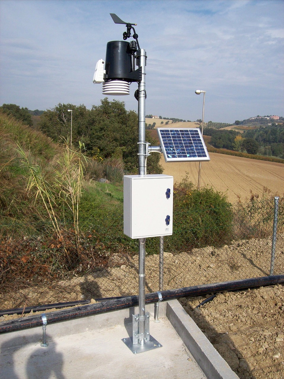
Precipitation has been measured for many centuries (Strangeways 2010). The traditional method is point measurement, which was standardized in the previous century to make measurements comparable in space and time. Fig. A2.5.3 shows a conventional weather station used to measure various weather-related parameters, including the amount of rainfall. Although statistical methods exist to calculate area averaged rainfall from weather stations, the limited number of data points remains a constraint, especially in developing countries and sparsely populated regions where the density of weather stations is low. Satellites can fill this information gap, as they observe the planet at a regular interval with calibrated sensors.
Fig. A2.5.3 Conventional weather station that measures various parameters, including precipitation |
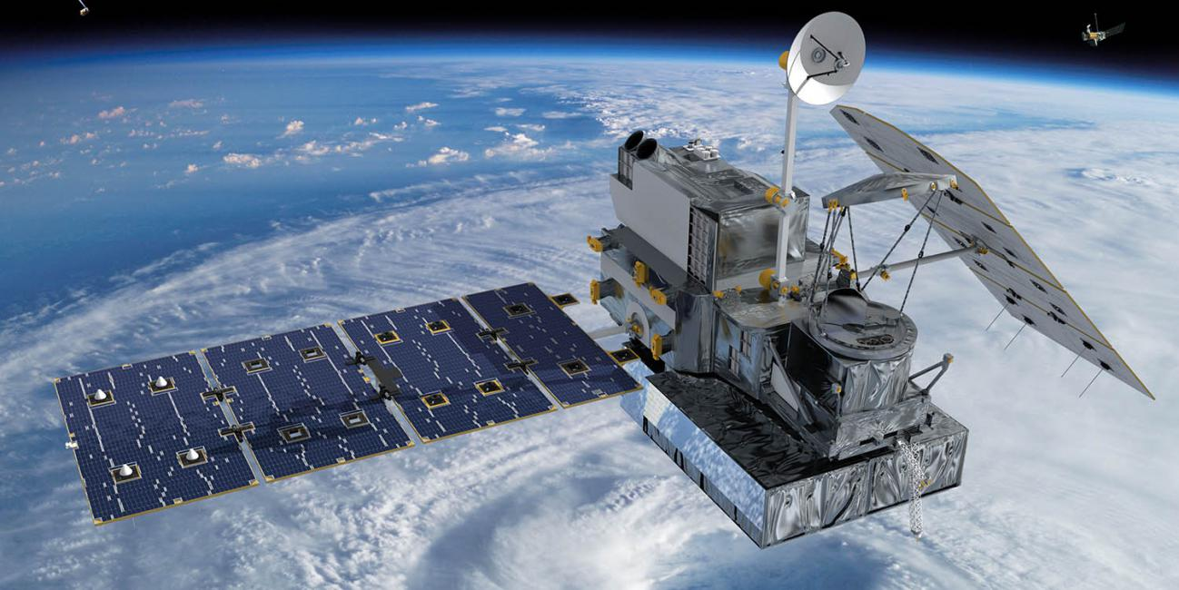
The Tropical Rainfall Measuring Mission (TRMM), a joint mission of the Japan Aerospace Exploration Agency (JAXA) and NASA, was a notable effort to monitor and study tropical rainfall (Kummerow et al. 1998). The satellite, which operated for 17 years, contained various instruments to measure clouds and cloud structures in order to advance understanding of the global energy and water cycles. The Global Precipitation Measurement (GPM; Fig. A2.5.4) mission is the successor, with the primary aim of making frequent (every 2–3 hours) observations of Earth's precipitation (Hou et al. 2014). A wide variety of data products are available for both TRMM and GPM. Precipitation estimates are derived from the Precipitation Radar (PR), TRMM Microwave Imager (TMI), Visible Infrared Scanner (VIRS), Clouds and Earth’s Radiant Energy System (CERES), and Lightning Imaging Sensor (LSI). Frequently used products of TRMM have a spatial resolution of 0.25 degrees (~25 km), whereas GPM has a higher resolution of 0.1 degrees (~10 km). Data is available on a three-hour time interval. The data can be obtained through NASA but also can be accessed from the Earth Engine data repository.
The Climate Hazards Group InfraRed Precipitation with Station (CHIRPS) data is a quasi-global rainfall dataset (Funk et al. 2015) covering more than 35 years. CHIRPS provides precipitation information at a 0.05 degrees (~5 km) spatial resolution. The dataset estimates precipitation by combining data from observing meteorological stations with satellite data. CHIRPS data is available at intervals from daily to annual and can be very valuable in hydrology studies, as it provides a long and consistent time series with precipitation estimates at a relatively high spatial resolution.
Fig. A2.5.4 The satellite for the Global Precipitation Measurement (GPM) mission |
Below is the code and an exercise to calculate monthly precipitation using these satellite data.
We begin by importing our area of interest, the Lower Mekong River Basin (Fig. A2.5.5).
// Import the Lower Mekong boundary. |
Fig. A2.5.5 The Lower Mekong Basin |
In the next step, we set the start and end dates for our analysis. We create a list for both years and months, which we will later use to iterate over.
// Set start and end years. |
We import the CHIRPS ImageCollection and select the imagery for the relevant dates, as presented in Chap. F4.2. Note that we used the pentad time series; each image in this collection contains the accumulated rainfall for five days. The daily product is also available in Earth Engine. The pentad dataset was used rather than the daily data product to reduce the number of computations needed to aggregate the data.
// Import the CHIRPS dataset. |
The year and month lists are used in the function below to calculate the monthly rainfall. We use a server-side nested loop where we first map over the years (2010, 2011, … 2020) and then map over the months (1, 2, … 12). This returns an image with the total rainfall for each month. We set the year, month, and timestamp ('system:time_start') for each image and flatten the image to turn the object into a single ImageCollection.
// We apply a nested loop where we first map over |
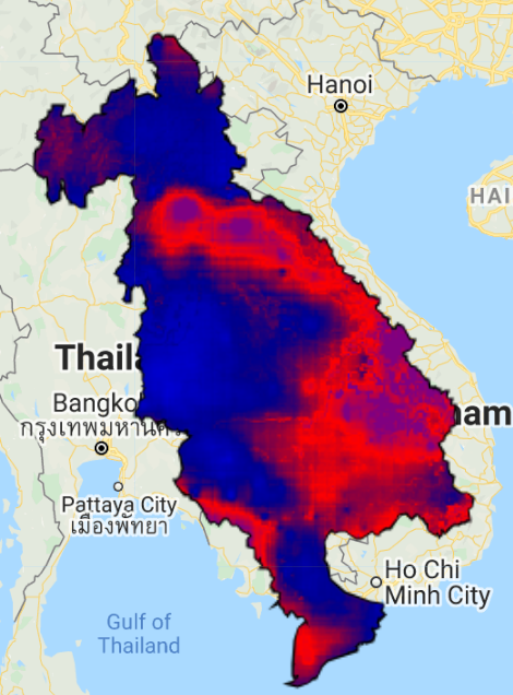
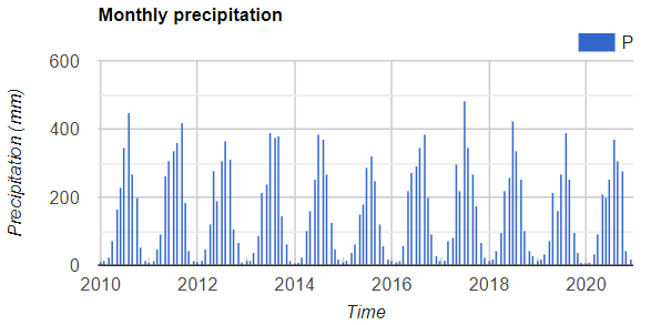
Add a layer with the monthly mean precipitation to the map and calculate a chart with monthly mean precipitation (Fig. A2.5.6).
// Add the layer with monthly mean. Note that we clip for the Mekong river basin. |
Fig. A2.5.6 Mean precipitation in the Lower Mekong Basin (left) and the monthly average precipitation (right) | |
Code Checkpoint A25a. The book’s repository contains a script that shows what your code should look like at this point.
Section 2. Calculating Monthly Evapotranspiration
Measuring evapotranspiration at large scales is important for assessing climate and anthropogenic effects on natural and agricultural ecosystems (Kustas and Norman 1996). Methods exist to measure ET at a field scale, but those methods cannot be extrapolated to larger areas. Traditional ways of estimating ET have been to use reference ET, derived from various weather-related parameters, with a crop coefficient. However, there are large uncertainties due to, for example, spatial and temporal heterogeneity and data gaps. Satellite information can be very useful as it provides spatially and temporally dense information for ET estimation.
Different methods exist to map ET from remote sensing data, including simple empirical models that relate spectral reflectance with ET, vegetation index models, energy budget, and deterministic models (Courault et al. 2005). Fundamentally, however, ET is governed by the energy budget and driving variables such as surface temperature. The total amount of available net radiant energy is divided into a soil heat flux and the atmospheric convective fluxes, which are the sensible heat flux (H) and latent energy exchanges (LE). This essentially means that the temperature decreases when energy is used for ET. Indeed, there are different ways to further quantify the different energy fluxes in more detail, and there is a wide body of scientific literature that describes those methods.
There are different readily available ET products derived from the Moderate Resolution Imaging Spectroradiometer (MODIS), including Atmosphere-Land Exchange Inverse (ALEXI; Anderson et al. 1997, Mecikalski et al. 1999), the operational Simplified Surface Energy Balance (SSEB; Senay et al. 2013), CSIRO MODIS Rescaled Evapotranspiration (CMRSET; Guerschman et al. 2009), and MOD16. The MOD16 algorithm is based on the logic of the Penman-Monteith equation, which uses daily meteorological reanalysis data and eight-day remotely sensed vegetation property dynamics from MODIS as inputs. The MOD16 product is available in the Earth Engine assets, and we will use this product for ET estimation in the next exercise.
First, we start a new script and repeat the first two steps of the previous section by copying and pasting the following code:
// Import the Lower Mekong boundary. |
We import the MOD16 dataset and select the ET band, which represents total evapotranspiration.
// Import the MOD16 dataset. |
We use the same function to calculate monthly values as in the previous section. Note that we multiply by 0.1 as a scaling factor. The scaling factor can be found in the description of the dataset in Earth Engine. Scaling factors are applied to reduce the required storage capacity by changing the data type.
// We apply a nested loop where we first map over |
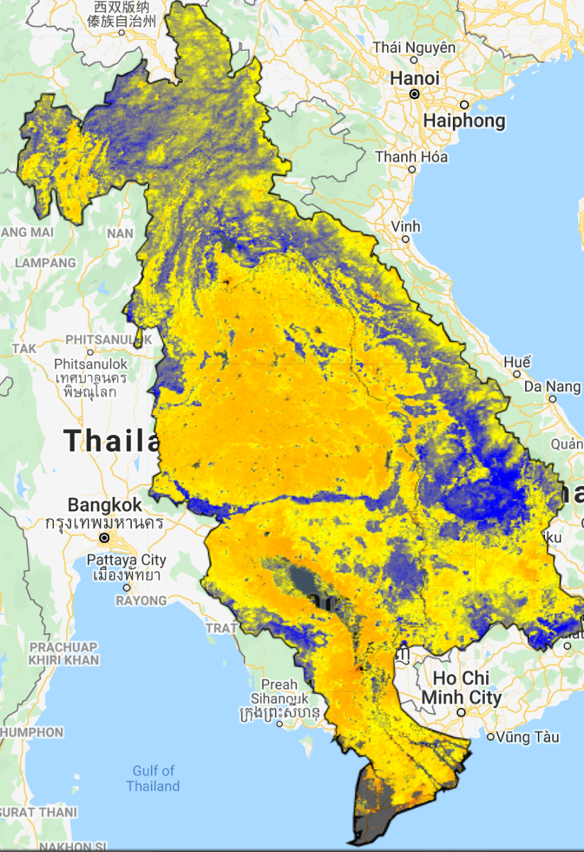
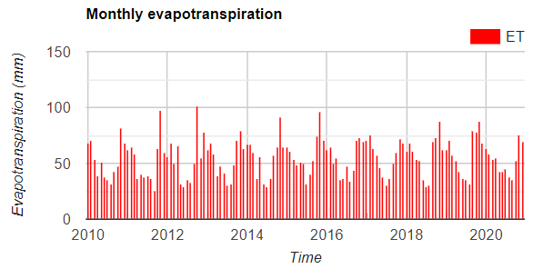
We use the code below to visualize the results. Note that we changed the color of the bar chart and applied the reducer on a 500 m spatial resolution.
// Add the layer with monthly mean. Note that we clip for the Mekong river basin. |
Fig. A2.5.7 Mean ET in the lower Mekong basin (left) and the monthly average ET (right) | |
Code Checkpoint A25b. The book’s repository contains a script that shows what your code should look like at this point.
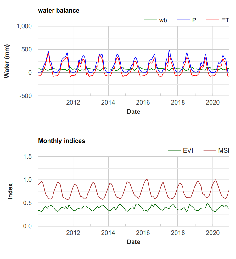
Section 3. Monthly Water Balance
We learned that the water balance is calculated using precipitation, evapotranspiration, runoff, and storage changes (Eq. A2.5.1). In the previous two sections, we calculated the monthly precipitation (P) on a 5 km spatial resolution and the monthly evapotranspiration (ET) on a 500 m spatial resolution. In Equation A2.5.2 we rearrange Equation 2.7.1 so that we can calculate the portion of Q and ΔS on a pixel level and aggregate that information to a basin level.
P − E =Q + ΔS (A2.5.2)
In this section we will use the previous data to calculate the monthly water balance. First, we set the dates and import the relevant ImageCollection, as shown in the previous sections. Copy and paste the code below in a new script.
// Import the Lower Mekong boundary. |
Now we use the function that we used earlier to calculate monthly ET and P to calculate the water balance.
// We apply a nested loop where we first map over |
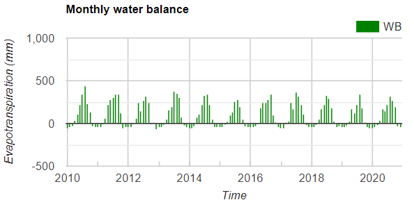
Next we add the monthly mean water balance to the map and calculate the monthly water balance (Fig. A2.5.8). Note that negative numbers in the map indicate regions with an overall surplus of ET, whereas negative monthly water balances indicate a surplus ET for the whole region.
// Add layer with monthly mean. note that we clip for the Mekong river basin. |
Fig. A2.5.8 Mean water balance in the lower Mekong basin (left) and the monthly average water balance (right) | |
Code Checkpoint A25c. The book’s repository contains a script that shows what your code should look like at this point.
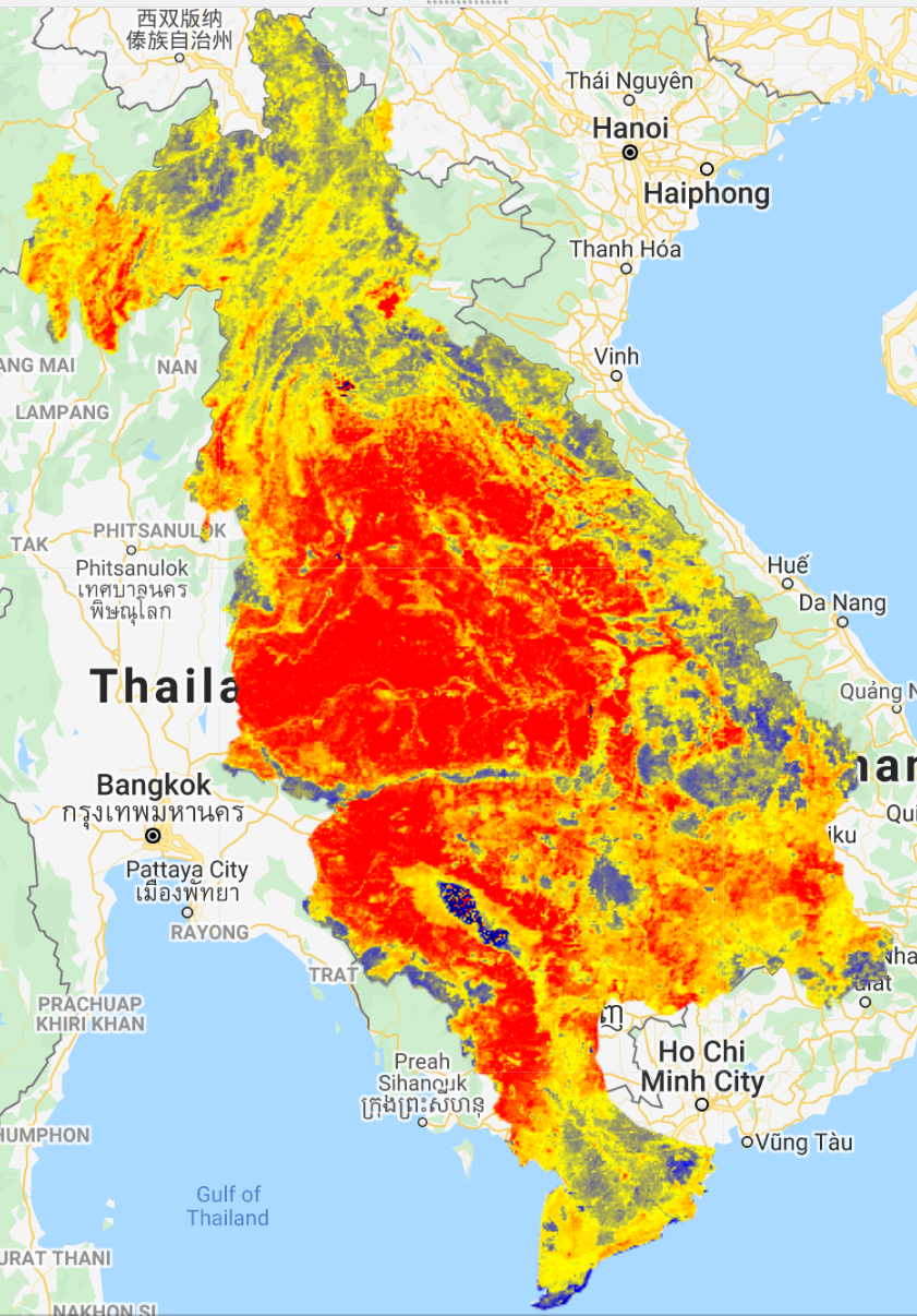
Section 4. Vegetation and Drought Indices
Calculating vegetation indices is a common practice when working with remote sensing data. The Normalized Difference Vegetation Index (NDVI; Rouse et al. 1973) and Enhanced Vegetation Index (EVI; Chap. F3.1) (Huete et al. 1994) are among the most commonly used. Vegetation indices rely on the absorption and reflection spectra of chlorophyll, often including the red band, where absorption is high, and near infrared, where reflection is high. Vegetation indices are often used to measure crop health and density, but they can also be used to measure, for example, biophysical health over longer time periods (Poortinga et al. 2018). Vegetation indices can be calculated from the spectral reflectance, but readily available products can be used as well. The latter have been processed and contain, for example, corrections for outliers and artifacts.
Besides vegetation indices, there are many other indices to describe specific natural phenomena or detect specific land surface features. These indices often rely on simple band ratios or more sophisticated formulas containing multiple bands. Drought indices are another category of important indicators as they enable us to depict spatiotemporal drought patterns in great detail. This can be particularly useful for remote areas where people rely on local agriculture for their livelihoods but production data is scarce. In the next exercise we will be using the Moisture Stress Index (MSI; Vogelmann 1985), as this index has been shown to be highly related to soil moisture. Eq. A2.5.3 shows that MSI is calculated from the shortwave infrared (SWIR) and near infrared (NIR) bands.
MSI=SWIR / NIR (A2.5.3)
In this section, we use the EVI product for the vegetation index from MODIS. This data is collected daily and can be used for calculation of the monthly vegetation index. You may note that we import the readily available EVI product and also import the spectral reflectance dataset.
We first import all the relevant datasets and define the period of interest, as in the other exercises, starting a new script.
// Import the Lower Mekong boundary. |
Two steps are needed to calculate the MSI. First, we need to remove the clouds and cloud shadows. This can be done by using the StateQA quality band that comes with the MOD09 product. After all the artifacts have been removed, we can calculate the MSI in the next function.
// We use a function to remove clouds and cloud shadows. |
We use the same nested loop as the previous sections, but now we calculate all layers and return an image where the layers are included as bands. Note that EVI and MOD16 are multiplied by the scale factor. For P, ET, and WB we calculate the sum; for MSI and EVI we calculate the mean.
// We apply a nested loop where we first map over |
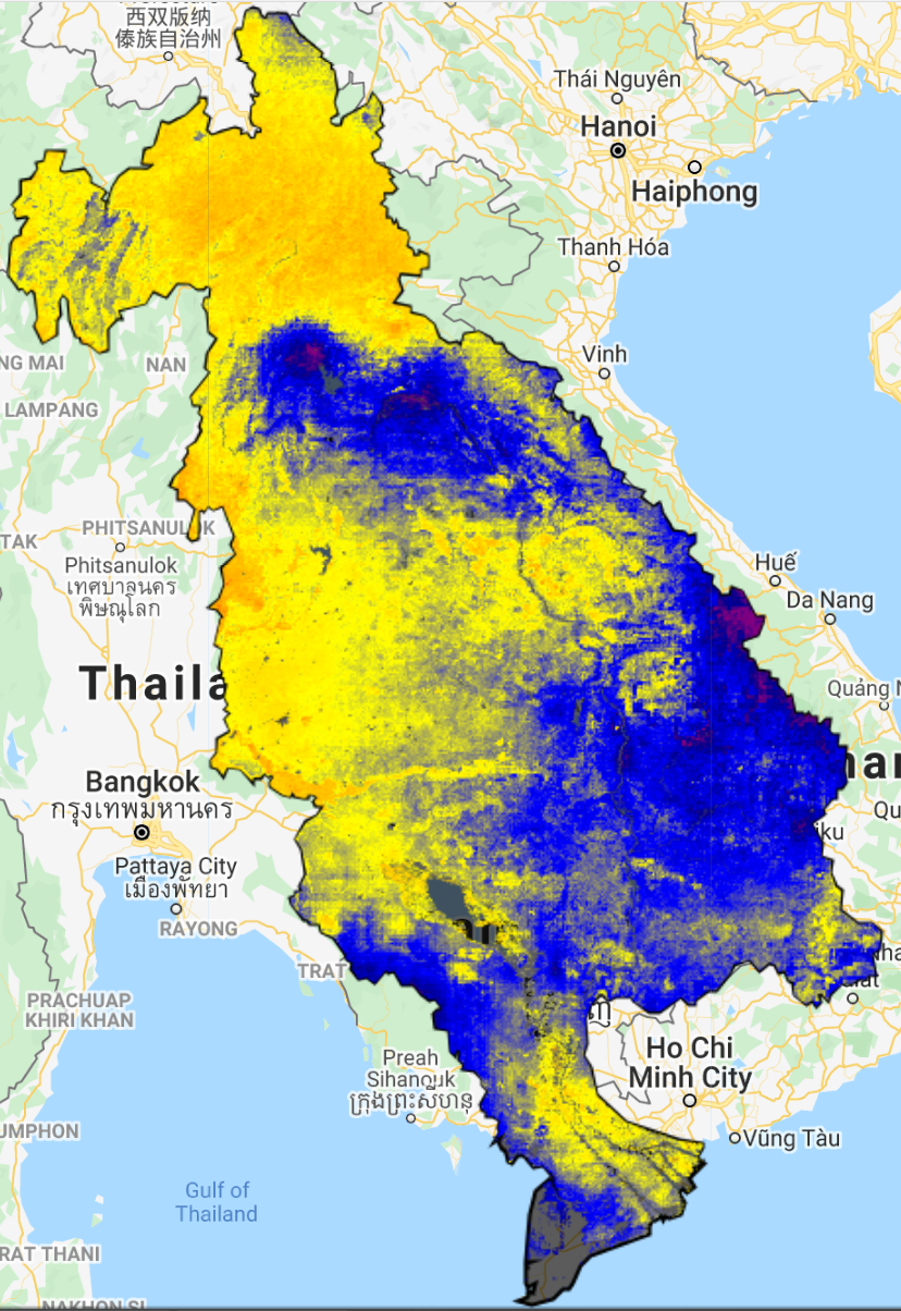
We display the monthly mean EVI and MSI and show the time series (Fig. A2.5.9).
// Add the mean monthly EVI and MSI to the map. |
Fig. A2.5.9 Monthly mean EVI (left), monthly mean MSI (middle), and the time series for the water balance (top right) and indices (bottom right) | ||

Code Checkpoint A25d. The book’s repository contains a script that shows what your code should look like at this point.
Section 5. Partitioning Water Resources and Mapping Drought Impacts
Historical and near-real-time remote-sensing-derived data can be very useful to assess the impact on the ground. For example, overlaying information layers on water resources with land cover information enables us to partition water resources by land cover and investigate consumptive use of, for example, different agricultural commodities. Overlaying land cover with vegetation and drought indicators helps to investigate land cover categories that are most impacted by water shortage. It also helps to assess the impacts on crop production and food security (Poortinga et al. 2019), as well as potential environmental impacts, including impacts on biodiversity. However, in many cases maps are produced and updated only infrequently and are often not accompanied by appropriate accuracy assessment information and documentation (Saah et al. 2019). Therefore, SERVIR-Mekong developed a time series of yearly land cover maps covering the greater Mekong region, including the Lower Mekong Basin (Saah et al. 2020, Potapov et al. 2019, Poortinga et al. 2020). Fig. A2.5.10 shows the land cover map of 2018.
Section 5.1. Annual Classifications
In the following subsections, we illustrate annual land cover maps and a variety of interpretations of them. The annual maps can be accessed using script A25s1 - Annual in the book repository.
Fig. A2.5.10 Land cover map of the Lower Mekong Basin |

Note: if you get an error related to “too many concurrent aggregations” in this last script link or the following ones, try re-running the script.
Section 5.2. Precipitation and Evapotranspiration
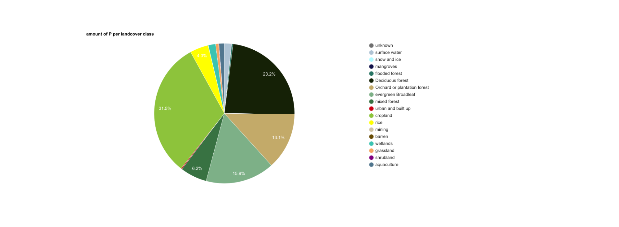
An example of partitioning water inputs and consumption is shown in Fig. A2.5.11. Here we calculate the mean P and ET for each land cover category using the land cover map. We can see that the largest portions of water are being used by cropland and agriculture; plantations also consume a large portion of the water. The pie charts can be created and viewed using script A25s2 - PET in the book repository.
Fig. A2.5.11 The amount of P (left) and ET (right) per land cover category | ||

Section 5.3. Monthly Water Balance
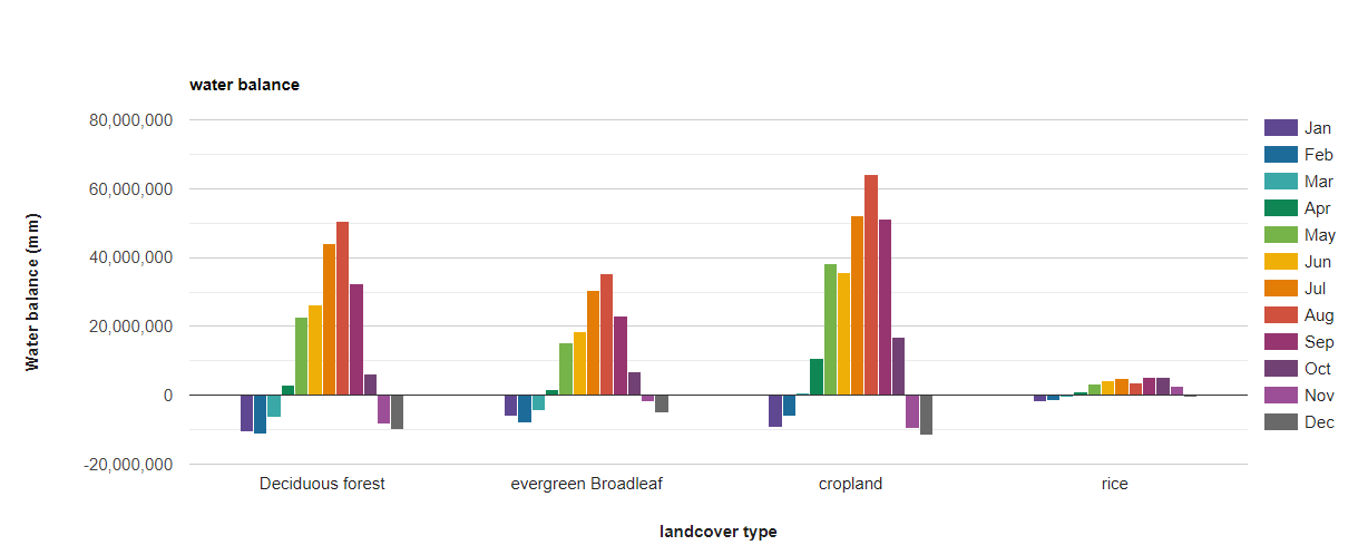
We can apply a similar overlaying method of partitioning for the water balance. Fig. A2.5.12 shows the monthly water balance for deciduous forest, evergreen broadleaf, cropland, and rice. It can be seen that a large portion of the water stored in the wet season is used by forest and cropland in the dry season. The area of paddy rice is smaller, so the total water consumption in the dry season of those categories is smaller. The monthly water balance charts can be found in script A25s3 - Monthly in the book repository.
Fig. A2.5.12 Water balance for four different land cover categories: deciduous forest, evergreen broadleaf, cropland, and rice |
Section 5.4. Per-class Water Balance Across Seasons
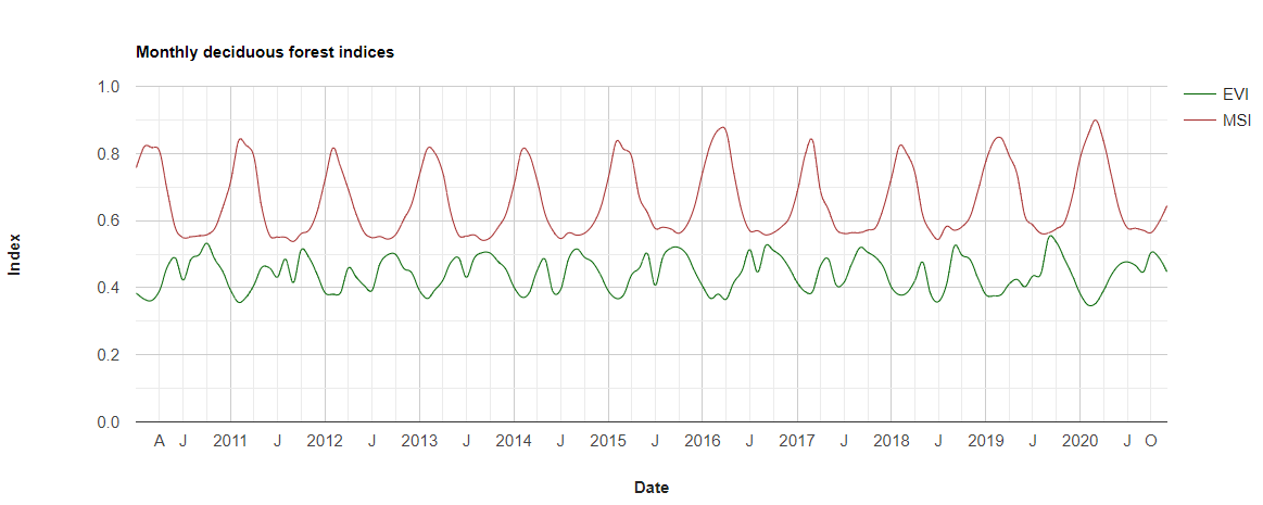
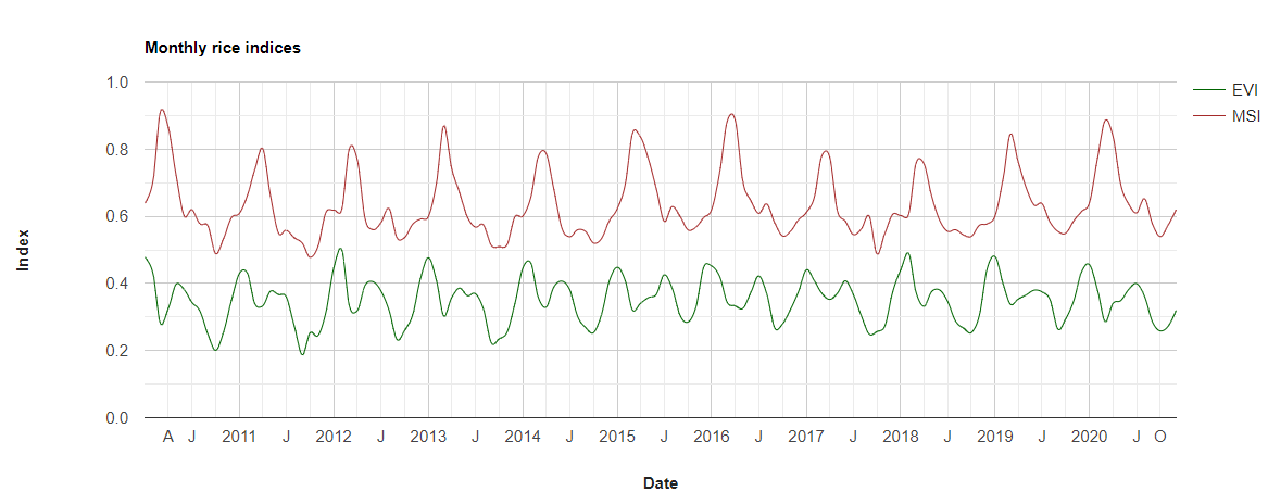
Partitioning can also be done per land cover category. In Fig. A2.5.13, we calculated the EVI and MSI for four land cover categories. There are very distinct patterns: we see little variation in the signal from the EVI, but large variations for the deciduous forest. For cropland, we found a signal that closely corresponds to the yearly dry and wet seasons, whereas we see multiple cropping seasons per year. The long time series enables us to investigate deviations from the mean, which in turn provides valuable information on, for example, potential drought impacts. The per-class water balance charts can be found in script A25s4 - Per Class Balance in the book repository.
Fig. A2.5.13 EVI and MSI per land cover category |


Synthesis
With what you learned in this chapter, you can analyze large-scale hydrological processes in a river basin. The approach can be applied for any river basin in the world using your own data or the open access data in the exercises.
Assignment 1. Test the approach in another part of the world using your own data or open-access data, or use your own training data for a more refined classification model.
Assignment 2. For further analysis, we encourage you to (1) replace MODIS with data from the Visible Infrared Imaging Radiometer Suite (VIIRS); (2) replace the CHIRPS data with the Integrated Multi-satellite Retrievals for GPM (IMERG) data and change the time intervals; and (3) use a different land cover map for partitioning the water resources.
Conclusion
A safe and sustainable supply of water is essential for drinking, washing, cleaning, cooking, and growing food. However, water is often a scarce resource that needs to be managed in a sustainable and equitable way. Satellite data products in Earth Engine can help us to map the quantity of water in space and time. It enables us to partition water according to its consumptive use and evaluate how this affects a wide variety of important functions within a water basin.
Feedback
To review this chapter and make suggestions or note any problems, please go now to bit.ly/EEFA-review. You can find summary statistics from past reviews at bit.ly/EEFA-reviews-stats.
References
Cloud-Based Remote Sensing with Google Earth Engine. (n.d.). CLOUD-BASED REMOTE SENSING WITH GOOGLE EARTH ENGINE. https://www.eefabook.org/
Cloud-Based Remote Sensing with Google Earth Engine. (2024). In Springer eBooks. https://doi.org/10.1007/978-3-031-26588-4
Anderson MC, Norman JM, Diak GR, et al (1997) A two-source time-integrated model for estimating surface fluxes using thermal infrared remote sensing. Remote Sens Environ 60:195–216. https://doi.org/10.1016/S0034-4257(96)00215-5
Courault D, Seguin B, Olioso A (2005) Review on estimation of evapotranspiration from remote sensing data: From empirical to numerical modeling approaches. Irrig Drain Syst 19:223–249. https://doi.org/10.1007/s10795-005-5186-0
Funk C, Peterson P, Landsfeld M, et al (2015) The climate hazards infrared precipitation with stations – a new environmental record for monitoring extremes. Sci Data 2:1–21. https://doi.org/10.1038/sdata.2015.66
Guerschman JP, Van Dijk AIJM, Mattersdorf G, et al (2009) Scaling of potential evapotranspiration with MODIS data reproduces flux observations and catchment water balance observations across Australia. J Hydrol 369:107–119. https://doi.org/10.1016/j.jhydrol.2009.02.013
Hou AY, Kakar RK, Neeck S, et al (2014) The global precipitation measurement mission. Bull Am Meteorol Soc 95:701–722. https://doi.org/10.1175/BAMS-D-13-00164.1
Huete A, Justice C, Liu H (1994) Development of vegetation and soil indices for MODIS-EOS. Remote Sens Environ 49:224–234. https://doi.org/10.1016/0034-4257(94)90018-3
Kummerow C, Barnes W, Kozu T, et al (1998) The tropical rainfall measuring mission (TRMM) sensor package. J Atmos Ocean Technol 15:809–817. https://doi.org/10.1175/1520-0426(1998)015<0809:TTRMMT>2.0.CO;2
Kustas WP, Norman JM (1996) Use of remote sensing for evapotranspiration monitoring over land surfaces. Hydrol Sci J 41:495–516. https://doi.org/10.1080/02626669609491522
Mecikalski JR, Diak GR, Anderson MC, Norman JM (1999) Estimating fluxes on continental scales using remotely sensed data in an atmospheric-land exchange model. J Appl Meteorol 38:1352–1369. https://doi.org/10.1175/1520-0450(1999)038<1352:EFOCSU>2.0.CO;2
Poortinga A, Aekakkararungroj A, Kityuttachai K, et al (2020) Predictive analytics for identifying land cover change hotspots in the Mekong region. Remote Sens 12:1472. https://doi.org/10.3390/RS12091472
Poortinga A, Clinton N, Saah D, et al (2018) An operational before-after-control-impact (BACI) designed platform for vegetation monitoring at planetary scale. Remote Sens 10:760. https://doi.org/10.3390/rs10050760
Poortinga A, Nguyen Q, Tenneson K, et al (2019) Linking Earth observations for assessing the food security situation in Vietnam: A landscape approach. Front Environ Sci 7:186. https://doi.org/10.3389/fenvs.2019.00186
Potapov P, Tyukavina A, Turubanova S, et al (2019) Annual continuous fields of woody vegetation structure in the Lower Mekong region from 2000‐2017 Landsat time-series. Remote Sens Environ 232:111278. https://doi.org/10.1016/j.rse.2019.111278
Rouse Jr JW, Haas RH, Schell JA, Deering DW (1973) Paper a 20. In: Third Earth Resources Technology Satellite-1 Symposium: Section AB. Technical presentations. pp 309
Saah D, Tenneson K, Matin M, et al (2019) Land cover mapping in data scarce environments: Challenges and opportunities. Front Environ Sci 7:150. https://doi.org/10.3389/fenvs.2019.00150
Saah D, Tenneson K, Poortinga A, et al (2020) Primitives as building blocks for constructing land cover maps. Int J Appl Earth Obs Geoinf 85:101979. https://doi.org/10.1016/j.jag.2019.101979
Senay GB, Bohms S, Singh RK, et al (2013) Operational evapotranspiration mapping using remote sensing and weather datasets: A new parameterization for the SSEB approach. J Am Water Resour Assoc 49:577–591. https://doi.org/10.1111/jawr.12057
Strangeways I (2010) A history of rain gauges. Weather 65:133–138. https://doi.org/10.1002/wea.548
Vogelmann JE, Rock BN (1985) Spectral characterization of suspected acid deposition damage in red spruce (Picea Rubens) stands from Vermont. In: Proc. of the Airborne Imaging Spectrometer Data Anal. Workshop.