Cloud-Based Remote Sensing with Google Earth Engine
Fundamentals and Applications

Part F4: Interpreting Image Series
One of the paradigm-changing features of Earth Engine is the ability to access decades of imagery without the previous limitation of needing to download all the data to a local disk for processing. Because remote-sensing data files can be enormous, this used to limit many projects to viewing two or three images from different periods. With Earth Engine, users can access tens or hundreds of thousands of images to understand the status of places across decades.
Chapter F4.1: Exploring Image Collections
Author
Gennadii Donchyts
Overview
This chapter teaches how to explore image collections, including their spatiotemporal extent, resolution, and values stored in images and image properties. You will learn how to map and inspect image collections using maps, charts, and interactive tools, and how to compute different statistics of values stored in image collections using reducers.
Learning Outcomes
- Inspecting the spatiotemporal extent and resolution of image collections by mapping image geometry and plotting image time properties.
- Exploring properties of images stored in an ImageCollection by plotting charts and deriving statistics.
- Filtering image collections by using stored or computed image properties.
- Exploring the distribution of values stored in image pixels of an ImageCollection through percentile reducers.
Assumes you know how to:
- Import images and image collections, filter, and visualize (Part F1).
- Perform basic image analysis: select bands, compute indices, create masks (Part F2).
- Summarize an ImageCollection with reducers (Chap. F4.0).
Github Code link for all tutorials
This code base is collection of codes that are freely available from different authors for google earth engine.
Practicum
In the previous chapter (Chap. F4.0), the filter, map, reduce paradigm was introduced. The main goal of this chapter is to demonstrate some of the ways that those concepts can be used within Earth Engine to better understand the variability of values stored in image collections. Sect. 1 demonstrates how time-dependent values stored in the images of an ImageCollection can be inspected using the Code Editor user interface after filtering them to a limited spatiotemporal range (i.e., geometry and time ranges). Sect. 2 shows how the extent of images, as well as basic statistics, such as the number of observations, can be visualized to better understand the spatiotemporal extent of image collections. Then, Sects. 3 and 4 demonstrate how simple reducers such as mean and median, and more advanced reducers such as percentiles, can be used to better understand how the values of a filtered ImageCollection are distributed.
Section 1. Filtering and Inspecting an Image Collection
We will focus on the area in and surrounding Lisbon, Portugal. Below, we will define a point, lisbonPoint, located in the city; access the very large Landsat ImageCollection and limit it to the year 2020 and to the images that contain Lisbon; and select bands 6, 5, and 4 from each of the images in the resulting filtered ImageCollection.
// Define a region of interest as a point in Lisbon, Portugal. |
The three selected bands (which correspond to SWIR1, NIR, and Red) display a false-color image that accentuates differences between different land covers (e.g., concrete, vegetation) in Lisbon. With the Inspector tab highlighted (Fig. F4.1.1), clicking on a point will bring up the values of bands 6, 5, and 4 from each of the images. If you open the Series option, you’ll see the values through time. For the specified point and for all other points in Lisbon (since they are all enclosed in the same Landsat scene), there are 16 images gathered in 2020. By following one of the graphed lines (in blue, yellow, or red) with your finger, you should be able to count that many distinct values. Moving the mouse along the lines will show the specific values and the image dates.
Fig. F4.1.1 Inspect values in an ImageCollection at a selected point by making use of the Inspector tool in the Code Editor |

We can also show this kind of chart automatically by making use of the ui.Chart function of the Earth Engine API. The following code snippet should result in the same chart as we could observe in the Inspector tab, assuming the same pixel is clicked.
// Construct a chart using values queried from image collection. |
Code Checkpoint F41a. The book’s repository contains a script that shows what your code should look like at this point.
Section 2. How Many Images Are There, Everywhere on Earth?
Suppose we are interested to find out how many valid observations we have at every map pixel on Earth for a given ImageCollection. This enormously computationally demanding task is surprisingly easy to do in Earth Engine. The API provides a set of reducer functions to summarize values to a single number in each pixel, as described in Chap. F4.0. We can apply this reducer, count, to our filtered ImageCollection with the code below. We’ll return to the same data set and filter for 2020, but without the geographic limitation. This will assemble images from all over the world, and then count the number of images in each pixel. The following code does that count, and adds the resulting image to the map with a predefined red/yellow/green color palette stretched between values 0 and 50. Continue pasting the code below into the same script.
// compute and show the number of observations in an image collection |
Run the command and zoom out. If the count of images over the entire Earth is viewed, the resulting map should look like Fig. F4.1.2. The created map data may take a few minutes to fully load in.
Fig. F4.1.2 The number of Landsat 8 images acquired during 2020 |
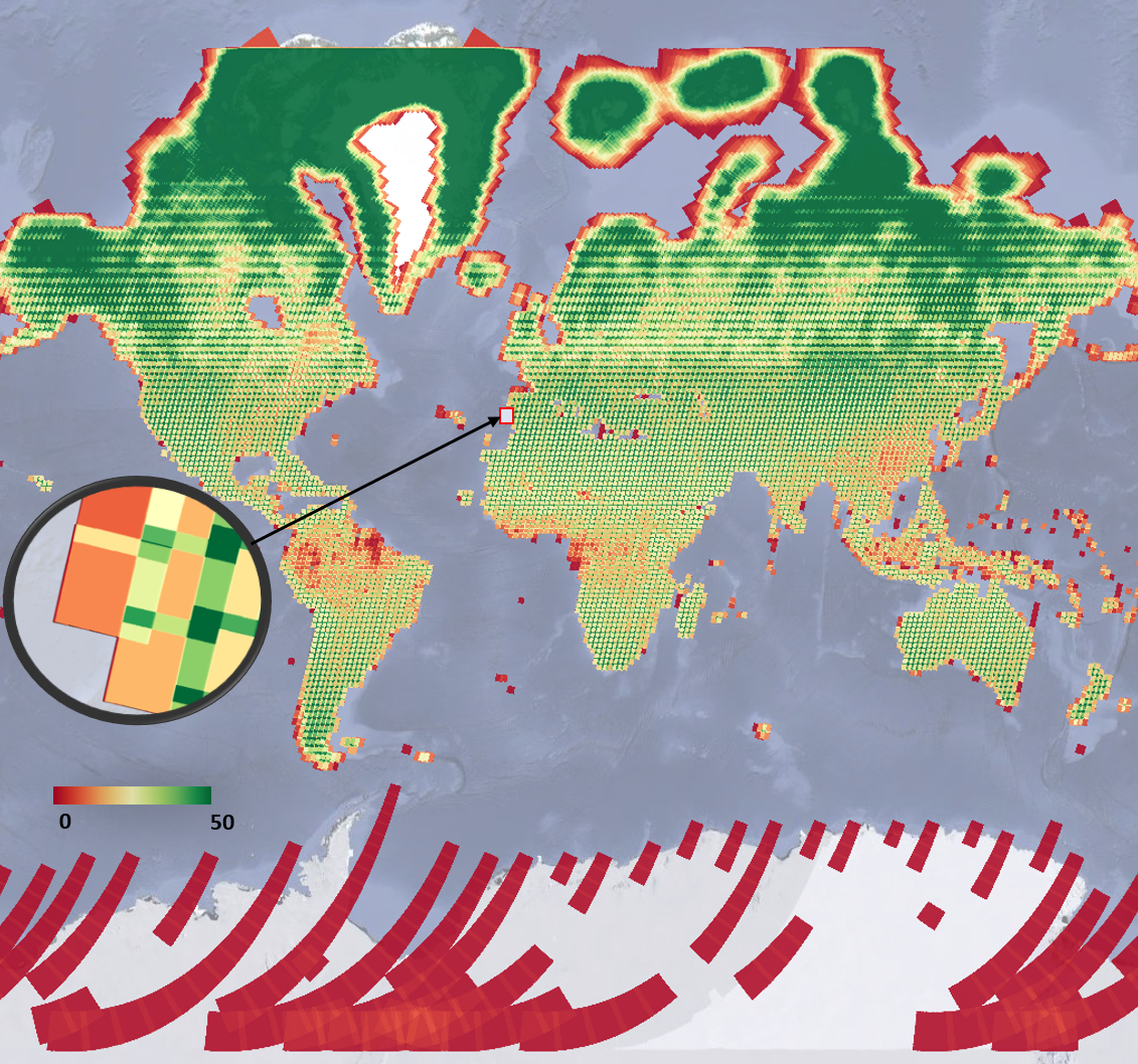
Note the checkered pattern, somewhat reminiscent of a Mondrian painting. To understand why the image looks this way, it is useful to consider the overlapping image footprints. As Landsat passes over, each image is wide enough to produce substantial “sidelap” with the images from the adjacent paths, which are collected at different dates according to the satellite’s orbit schedule. In the north-south direction, there is also some overlap to ensure that there are no gaps in the data. Because these are served as distinct images and stored distinctly in Earth Engine, you will find that there can be two images from the same day with the same value for points in these overlap areas. Depending on the purposes of a study, you might find a way to ignore the duplicate pixel values during the analysis process.
You might have noticed that we summarized a single band from the original ImageCollection to ensure that the resulting image would give a single count in each pixel. The count reducer operates on every band passed to it. Since every image has the same number of bands, passing an ImageCollection of all seven Landsat bands to the count reducer would have returned seven identical values of 16 for every point. To limit any confusion from seeing the same number seven times, we selected one of the bands from each image in the collection. In your own work, you might want to use a different reducer, such as a median operation, that would give different, useful answers for each band. A few of these reducers are described below.
Code Checkpoint F41b. The book’s repository contains a script that shows what your code should look like at this point.
Section 3. Reducing Image Collections to Understand Band Values
As we have seen, you could click at any point on Earth’s surface and see both the number of Landsat images recorded there in 2020 and the values of any image in any band through time. This is impressive and perhaps mind-bending, given the enormous amount of data in play. In this section and the next, we will explore two ways to summarize the numerical values of the bands—one straightforward way and one more complex but highly powerful way to see what information is contained in image collections.
First, we will make a new layer that represents the mean value of each band in every pixel across every image from 2020 for the filtered set, add this layer to the layer set, and explore again with the Inspector. The previous section’s count reducer was called directly using a sort of simple shorthand; that could be done similarly here by calling mean on the assembled bands. In this example, we will use the reducer to get the mean using the more general reduce call. Continue pasting the code below into the same script.
// Zoom to an informative scale for the code that follows. |
Now, let’s look at the median value for each band among all the values gathered in 2020. Using the code below, calculate the median and explore the image with the Inspector. Compare this image briefly to the mean image by eye and by clicking in a few pixels in the Inspector. They should have different values, but in most places they will look very similar.
// Add a median composite image. |
There is a wide range of reducers available in Earth Engine. If you are curious about which reducers can be used to summarize band values across a collection of images, use the Docs tab in the Code Editor to list all reducers and look for those beginning with ee.Reducer.
Code Checkpoint F41c. The book’s repository contains a script that shows what your code should look like at this point.
Section 4. Compute Multiple Percentile Images for an Image Collection
One particularly useful reducer that can help you better understand the variability of values in image collections is ee.Reducer.percentile. The nth percentile gives the value that is the nth largest in a set. In this context, you can imagine accessing all of the values for a given band in a given ImageCollection for a given pixel and sorting them. The 30th percentile, for example, is the value 30% of the way along the list from smallest to largest. This provides an easy way to explore the variability of the values in image collections by computing a cumulative density function of values on a per-pixel basis. The following code shows how we can calculate a single 30th percentile on a per-pixel and per-band basis for our Landsat 8 ImageCollection. Continue pasting the code below into the same script.
// compute a single 30% percentile |
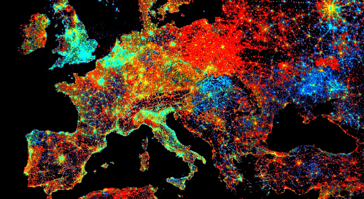
Fig. F4.1.3 Landsat 8 TOA reflectance 30th percentile image computed for ImageCollection with images acquired during 2020 |

We can see that the resulting composite image (Fig. 4.1.3) has almost no cloudy pixels present for this area. This happens because cloudy pixels usually have higher reflectance values. At the lowest end of the values, other unwanted effects like cloud or hill shadows typically have very low reflectance values. This is why this 30th percentile composite image looks so much cleaner than the mean composite image (meanFilteredIC) calculated earlier. Note that the reducers operate per pixel: adjacent pixels are drawn from different images. This means that one pixel’s value could be taken from an image from one date, and the adjacent pixel’s value drawn from an entirely different period. Although, like the mean and median images, percentile images such as that seen in Fig. F4.1.3 never existed on a single day, composite images allow us to view Earth’s surface without the noise that can make analysis difficult.
We can explore the range of values in an entire ImageCollection by viewing a series of increasingly bright percentile images, as shown in Fig. F4.1.4. Paste and run the following code.
var percentiles=[0, 10, 20, 30, 40, 50, 60, 70, 80]; |
Note that the code adds every percentile image as a separate map layer, so you need to go to the Layers control and show/hide different layers to explore differences. Here, we can see that low-percentile composite images depict darker, low-reflectance land features, such as water and cloud or hill shadows, while higher-percentile composite images (>70% in our example) depict clouds and any other atmospheric or land effects corresponding to bright reflectance values.
Fig. F4.1.4 Landsat 8 TOA reflectance percentile composite images |

Earth Engine provides a very rich API, allowing users to explore image collections to better understand the extent and variability of data in space, time, and across bands, as well as tools to analyze values stored in image collections in a frequency domain. Exploring these values in different forms should be the first step of any study before developing data analysis algorithms.
Code Checkpoint F41d. The book’s repository contains a script that shows what your code should look like at this point.
Synthesis
In the example above, the 30th percentile composite image would be useful for typical studies that need cloud-free data for analysis. The “best” composite to use, however, will depend on the goal of a study, the characteristics of the given data set, and the location being viewed. You can imagine choosing different percentile composite values if exploring image collections over the Sahara Desert or over Congo, where cloud frequency would vary substantially (Wilson et al. 2016).
Assignment 1. Noting that your own interpretation of what constitutes a good composite is subjective, create a series of composites of a different location, or perhaps a pair of locations, for a given set of dates.
Assignment 2. Filter to create a relevant data set—for example, for Landsat 8 or Sentinel-2 over an agricultural growing season. Create percentile composites for a given location. Which image composite is the most satisfying, and what type of project do you have in mind when giving that response?
Assignment 3. Do you think it is possible to generalize about the relationship between the time window of an ImageCollection and the percentile value that will be the most useful for a given project, or will every region need to be inspected separately?
Conclusion
In this chapter, you have learned different ways to explore image collections using Earth Engine in addition to looking at individual images. You have learned that image collections in Earth Engine may have global footprints as well as images with a smaller, local footprint, and how to visualize the number of images in a given filtered ImageCollection. You have learned how to explore the temporal and spatial extent of images stored in image collections, and how to quickly examine the variability of values in these image collections by computing simple statistics like mean or median, as well as how to use a percentile reducer to better understand this variability.
Feedback
To review this chapter and make suggestions or note any problems, please go now to bit.ly/EEFA-review. You can find summary statistics from past reviews at bit.ly/EEFA-reviews-stats.
References
Cloud-Based Remote Sensing with Google Earth Engine. (n.d.). CLOUD-BASED REMOTE SENSING WITH GOOGLE EARTH ENGINE. https://www.eefabook.org/
Cloud-Based Remote Sensing with Google Earth Engine. (2024). In Springer eBooks. https://doi.org/10.1007/978-3-031-26588-4
Wilson AM, Jetz W (2016) Remotely sensed high-resolution global cloud dynamics for predicting ecosystem and biodiversity distributions. PLoS Biol 14:e1002415. https://doi.org/10.1371/journal.pbio.1002415