Cloud-Based Remote Sensing with Google Earth Engine
Fundamentals and Applications

Part F4: Interpreting Image Series
One of the paradigm-changing features of Earth Engine is the ability to access decades of imagery without the previous limitation of needing to download all the data to a local disk for processing. Because remote-sensing data files can be enormous, this used to limit many projects to viewing two or three images from different periods. With Earth Engine, users can access tens or hundreds of thousands of images to understand the status of places across decades.
Chapter F4.0: Filter, Map, Reduce
Author
Jeffrey A. Cardille
Overview
The purpose of this chapter is to teach you important programming concepts as they are applied in Earth Engine. We first illustrate how the order and type of these operations can matter with a real-world, non-programming example. We then demonstrate these concepts with an ImageCollection, a key data type that distinguishes Earth Engine from desktop image-processing implementations.
Learning Outcomes
- Visualizing the concepts of filtering, mapping, and reducing with a hypothetical, non-programming example.
- Gaining context and experience with filtering an ImageCollection.
- Learning how to efficiently map a user-written function over the images of a filtered ImageCollection.
- Learning how to summarize a set of assembled values using Earth Engine reducers.
Assumes you know how to:
- Import images and image collections, filter, and visualize (Part F1).
- Perform basic image analysis: select bands, compute indices, create masks (Part F2).
Github Code link for all tutorials
This code base is collection of codes that are freely available from different authors for google earth engine.
Introduction to Theory
Prior chapters focused on exploring individual images—for example, viewing the characteristics of single satellite images by displaying different combinations of bands (Chap. F1.1), viewing single images from different datasets (Chap. F1.2, Chap. F1.3), and exploring image processing principles (Parts F2, F3) as they are implemented for cloud-based remote sensing in Earth Engine. Each image encountered in those chapters was pulled from a larger assemblage of images taken from the same sensor. The chapters used a few ways to narrow down the number of images in order to view just one for inspection (Part F1) or manipulation (Part F2, Part F3).
In this chapter and most of the chapters that follow, we will move from the domain of single images to the more complex and distinctive world of working with image collections, one of the fundamental data types within Earth Engine. The ability to conceptualize and manipulate entire image collections distinguishes Earth Engine and gives it considerable power for interpreting change and stability across space and time.
When looking for change or seeking to understand differences in an area through time, we often proceed through three ordered stages, which we will color code in this first explanatory part of the lab:
- Filter: selecting subsets of images based on criteria of interest.
- Map: manipulating each image in a set in some way to suit our goals. and
- Reduce: estimating characteristics of the time series.
For users of other programming languages—R, MATLAB, C, Karel, and many others—this approach might seem awkward at first. We explain it below with a non-programming example: going to the store to buy milk.
Suppose you need to go shopping for milk, and you have two criteria for determining where you will buy your milk: location and price. The store needs to be close to your home, and as a first step in deciding whether to buy milk today, you want to identify the lowest price among those stores. You don’t know the cost of milk at any store ahead of time, so you need to efficiently contact each one and determine the minimum price to know whether it fits in your budget. If we were discussing this with a friend, we might say, “I need to find out how much milk costs at all the stores around here.” To solve that problem in a programming language, these words imply precise operations on sets of information. We can write the following “pseudocode,” which uses words that indicate logical thinking but that cannot be pasted directly into a program:
AllStoresOnEarth.filterNearbyStores.filterStoresWithMilk.getMilkPricesFromEachStore.determineTheMinimumValue
Imagine doing these actions not on a computer but in a more old-fashioned way: calling on the telephone for milk prices, writing the milk prices on paper, and inspecting the list to find the lowest value. In this approach, we begin with AllStoresOnEarth, since there is at least some possibility that we could decide to visit any store on Earth, a set that could include millions of stores, with prices for millions or billions of items. A wise first action would be to limit ourselves to nearby stores. Asking to filterNearbyStores would reduce the number of potential stores to hundreds, depending on how far we are willing to travel for milk. Then, working with that smaller set, we further filterStoresWithMilk, limiting ourselves to stores that sell our target item. At that point in the filtering, imagine that just 10 possibilities remain. Then, by telephone, we getMilkPricesFromEachStore, making a short paper list of prices. We then scan the list to determineTheMinimumValue to decide which store to visit.
In that example, each color plays a different role in the workflow. The AllStoresOnEarth set, any one of which might contain inexpensive milk, is an enormous collection. The filtering actions filterNearbyStores and filterStoresWithMilk are operations that can happen on any set of stores. These actions take a set of stores, do some operation to limit that set, and return that smaller set of stores as an answer. The action to getMilkPricesFromEachStore takes a simple idea—calling a store for a milk price—and “maps” it over a given set of stores. Finally, with the list of nearby milk prices assembled, the action to determineTheMinimumValue, a general idea that could be applied to any list of numbers, identifies the cheapest one.
The list of steps above might seem almost too obvious, but the choice and order of operations can have a big impact on the feasibility of the problem. Imagine if we had decided to do the same operations in a slightly different order:
AllStoresOnEarth.filterStoresWithMilk.getMilkPricesFromEachStore.filterNearbyStores.determineMinimumValue
In this approach, we first identify all the stores on Earth that have milk, then contact them one by one to get their current milk price. If the contact is done by phone, this could be a painfully slow process involving millions of phone calls. It would take considerable “processing” time to make each call, and careful work to record each price onto a giant list. Processing the operations in this order would demand that only after entirely finishing the process of contacting every milk proprietor on Earth, we then identify the ones on our list that are not nearby enough to visit, then scan the prices on the list of nearby stores to find the cheapest one. This should ultimately give the same answer as the more efficient first example, but only after requiring so much effort that we might want to give up.
In addition to the greater order of magnitude of the list size, you can see that there are also possible slow points in the process. Could you make a million phone calls yourself? Maybe, but it might be pretty appealing to hire, say, 1000 people to help. While being able to make a large number of calls in parallel would speed up the calling stage, it’s important to note that you would need to wait for all 1000 callers to return their sublists of prices. Why wait? Nearby stores could be on any caller’s sublist, so any caller might be the one to find the lowest nearby price. The identification of the lowest nearby price would need to wait for the slowest caller, even if it turned out that all of that last caller’s prices came from stores on the other side of the world.
This counterexample would also have other complications—such as the need to track store locations on the list of milk prices—that could present serious problems if you did those operations in that unwise order. For now, the point is to filter, then map, then reduce. Below, we’ll apply these concepts to image collections.
Practicum
Section 1. Filtering Image Collections in Earth Engine
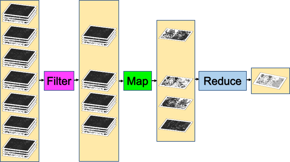
The first part of the filter, map, reduce paradigm is “filtering” to get a smaller ImageCollection from a larger one. As in the milk example, filters take a large set of items, limit it by some criterion, and return a smaller set for consideration. Here, filters take an ImageCollection, limit it by some criterion of date, location, or image characteristics, and return a smaller ImageCollection (Fig. F4.0.1).
Fig. 4.0.1 Filter, map, reduce as applied to image collections in Earth Engine |
As described first in Chap. F1.2, the Earth Engine API provides a set of filters for the ImageCollection type. The filters can limit an ImageCollection based on spatial, temporal, or attribute characteristics. Filters were used in Parts F1, F2, and F3 without much context or explanation, to isolate an image from an ImageCollection for inspection or manipulation. The information below should give perspective on that work while introducing some new tools for filtering image collections.
Below are three examples of limiting a Landsat 5 ImageCollection by characteristics and assessing the size of the resulting set.
FilterDate This takes an ImageCollection as input and returns an ImageCollection whose members satisfy the specified date criteria. We’ll adapt the earlier filtering logic seen in Chap. F1.2:
var imgCol=ee.ImageCollection('LANDSAT/LT05/C02/T1_L2'); |
After running the code, you should get a very large number for the full set of images. You also will likely get a very large number for the subset of images over the decade-scale interval.
FilterBounds It may be that—similar to the milk example—only images near to a place of interest are useful for you. As first presented in Part F1, filterBounds takes an ImageCollection as input and returns an ImageCollection whose images surround a specified location. If we take the ImageCollection that was filtered by date and then filter it by bounds, we will have filtered the collection to those images near a specified point within the specified date interval. With the code below, we’ll count the number of images in the Shanghai vicinity, first visited in Chap. F1.1, from the early 2000s:
var ShanghaiImage=ee.Image( |
If you’d like, you could take a few minutes to explore the behavior of the script in different parts of the world. To do that, you would need to comment out the Map.centerObject command to keep the map from moving to that location each time you run the script.
Filter by Other Image Metadata As first explained in Chap. F1.3, the date and location of an image are characteristics stored with each image. Another important factor in image processing is the cloud cover, an image-level value computed for each image in many collections, including the Landsat and Sentinel-2 collections. The overall cloudiness score might be stored under different metadata tag names in different data sets. For example, for Sentinel-2, this overall cloudiness score is stored in the CLOUDY_PIXEL_PERCENTAGE metadata field. For Landsat 5, the ImageCollection we are using in this example, the image-level cloudiness score is stored using the tag CLOUD_COVER. If you are unfamiliar with how to find this information, these skills are first presented in Part F1.
Here, we will access the ImageCollection that we just built using filterBounds and filterDate, and then further filter the images by the image-level cloud cover score, using the filterMetadata function.
Next, let’s remove any images with 50% or more cloudiness. As will be described in subsequent chapters working with per-pixel cloudiness information, you might want to retain those images in a real-life study, if you feel some values within cloudy images might be useful. For now, to illustrate the filtering concept, let’s keep only images whose image-level cloudiness values indicate that the cloud coverage is lower than 50%. Here, we will take the set already filtered by bounds and date, and further filter it using the cloud percentage into a new ImageCollection. Add this line to the script to filter by cloudiness and print the size to the Console.
var L5FilteredLowCloudImages=imgColfilteredByDateHere |
Filtering in an Efficient Order As you saw earlier in the hypothetical milk example, we typically filter, then map, and then reduce, in that order. In the same way that we would not want to call every store on Earth, preferring instead to narrow down the list of potential stores first, we filter images first in our workflow in Earth Engine. In addition, you may have noticed that the ordering of the filters within the filtering stage also mattered in the milk example. This is also true in Earth Engine. For problems with a non-global spatial component in which filterBounds is to be used, it is most efficient to do that spatial filtering first.
In the code below, you will see that you can “chain” the filter commands, which are then executed from left to right. Below, we chain the filters in the same order as you specified above. Note that it gives an ImageCollection of the same size as when you applied the filters one at a time.
var chainedFilteredSet=imgCol.filterDate(startDate, endDate) |
In the code below, we chain the filters in a more efficient order, implementing filterBounds first. This, too, gives an ImageCollection of the same size as when you applied the filters in the less efficient order, whether the filters were chained or not.
var efficientFilteredSet=imgCol.filterBounds(Map.getCenter()) |
Each of the two chained sets of operations will give the same result as before for the number of images. While the second order is more efficient, both approaches are likely to return the answer to the Code Editor at roughly the same time for this very small example. The order of operations is most important in larger problems in which you might be challenged to manage memory carefully. As in the milk example in which you narrowed geographically first, it is good practice in Earth Engine to order the filters with the filterBounds first, followed by metadata filters in order of decreasing specificity.
Code Checkpoint F40a. The book’s repository contains a script that shows what your code should look like at this point.
Now, with an efficiently filtered collection that satisfies our chosen criteria, we will next explore the second stage: executing a function for all of the images in the set.
Section 2. Mapping over Image Collections in Earth Engine
In Chap. F3.1, we calculated the Enhanced Vegetation Index (EVI) in very small steps to illustrate band arithmetic on satellite images. In that chapter, code was called once, on a single image. What if we wanted to compute the EVI in the same way for every image of an entire ImageCollection? Here, we use the key tool for the second part of the workflow in Earth Engine, a .map command (Fig. F4.0.1). This is roughly analogous to the step of making phone calls in the milk example that began this chapter, in which you took a list of store names and transformed it through effort into a list of milk prices.
Before beginning to code the EVI functionality, it’s worth noting that the word “map” is encountered in multiple settings during cloud-based remote sensing, and it’s important to be able to distinguish the uses. A good way to think of it is that “map” can act as a verb or as a noun in Earth Engine. There are two uses of “map” as a noun. We might refer casually to “the map,” or more precisely to “the Map panel”; these terms refer to the place where the images are shown in the code interface. A second way “map” is used as a noun is to refer to an Earth Engine object, which has functions that can be called on it. Examples of this are the familiar Map.addLayer and Map.setCenter. Where that use of the word is intended, it will be shown in purple text and capitalized in the Code Editor. What we are discussing here is the use of .map as a verb, representing the idea of performing a set of actions repeatedly on a set. This is typically referred to as “mapping over the set.”
To map a given set of operations efficiently over an entire ImageCollection, the processing needs to be set up in a particular way. Users familiar with other programming languages might expect to see “loop” code to do this, but the processing is not done exactly that way in Earth Engine. Instead, we will create a function, and then map it over the ImageCollection. To begin, envision creating a function that takes exactly one parameter, an ee.Image. The function is then designed to perform a specified set of operations on the input ee.Image and then, importantly, returns an ee.Image as the last step of the function. When we map that function over an ImageCollection, as we’ll illustrate below, the effect is that we begin with an ImageCollection, do operations to each image, and receive a processed ImageCollection as the output.
What kinds of functions could we create? For example, you could imagine a function taking an image and returning an image whose pixels have the value 1 where the value of a given band was lower than a certain threshold, and 0 otherwise. The effect of mapping this function would be an entire ImageCollection of images with zeroes and ones representing the results of that test on each image. Or you could imagine a function computing a complex self-defined index and sending back an image of that index calculated in each pixel. Here, we’ll create a function to compute the EVI for any input Landsat 5 image and return the one-band image for which the index is computed for each pixel. Copy and paste the function definition below into the Code Editor, adding it to the end of the script from the previous section.
var makeLandsat5EVI=function(oneL5Image){ |
It is worth emphasizing that, in general, band names are specific to each ImageCollection. As a result, if that function were run on an image without the band 'SR_B4', for example, the function call would fail. Here, we have emphasized in the function’s name that it is specifically for creating EVI for Landsat 5.
The function makeLandsat5EVI is built to receive a single image, select the proper bands for calculating EVI, make the calculation, and return a one-banded image. If we had the name of each image comprising our ImageCollection, we could enter the names into the Code Editor and call the function one at a time for each, assembling the images into variables, and then combining them into an ImageCollection. This would be very tedious and highly prone to mistakes: lists of items might get mistyped, an image might be missed, etc. Instead, as mentioned above, we will use .map. With the code below, let’s print the information about the cloud-filtered collection and display it, execute the .map command, and explore the resulting ImageCollection.
var L5EVIimages=efficientFilteredSet.map(makeLandsat5EVI); |
After entering and executing this code, you will see a grayscale image. If you look closely at the edges of the image, you might spot other images drawn behind it in a way that looks somewhat like a stack of papers on a table. This is the drawing of the ImageCollection made from the makeLandsat5EVI function. You can select the Inspector panel and click on one of the grayscale pixels to view the values of the entire ImageCollection. After clicking on a pixel, look for the Series tag by opening and closing the list of items. When you open that tag, you will see a chart of the EVI values at that pixel, created by mapping the makeLandsat5EVI function over the filtered ImageCollection.
Code Checkpoint F40b. The book’s repository contains a script that shows what your code should look like at this point.
Section 3. Reducing an Image Collection
The third part of the filter, map, reduce paradigm is “reducing” values in an ImageCollection to extract meaningful values (Fig. F4.0.1). In the milk example, we reduced a large list of milk prices to find the minimum value. The Earth Engine API provides a large set of reducers for reducing a set of values to a summary statistic.
Here, you can think of each location, after the calculation of EVI has been executed though the .map command, as having a list of EVI values on it. Each pixel contains a potentially very large set of EVI values; the stack might be 15 items high in one location and perhaps 200, 2000, or 200,000 items high in another location, especially if a looser set of filters had been used.
The code below computes the mean value, at every pixel, of the ImageCollection L5EVIimages created above. Add it at the bottom of your code.
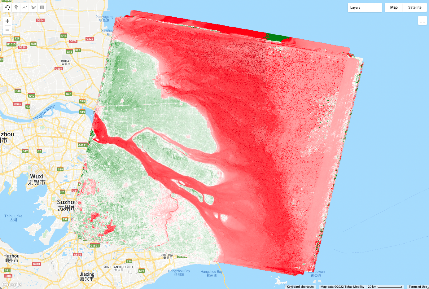
var L5EVImean=L5EVIimages.reduce(ee.Reducer.mean()); |
Using the same principle, the code below computes and draws the median value of the ImageCollection in every pixel.
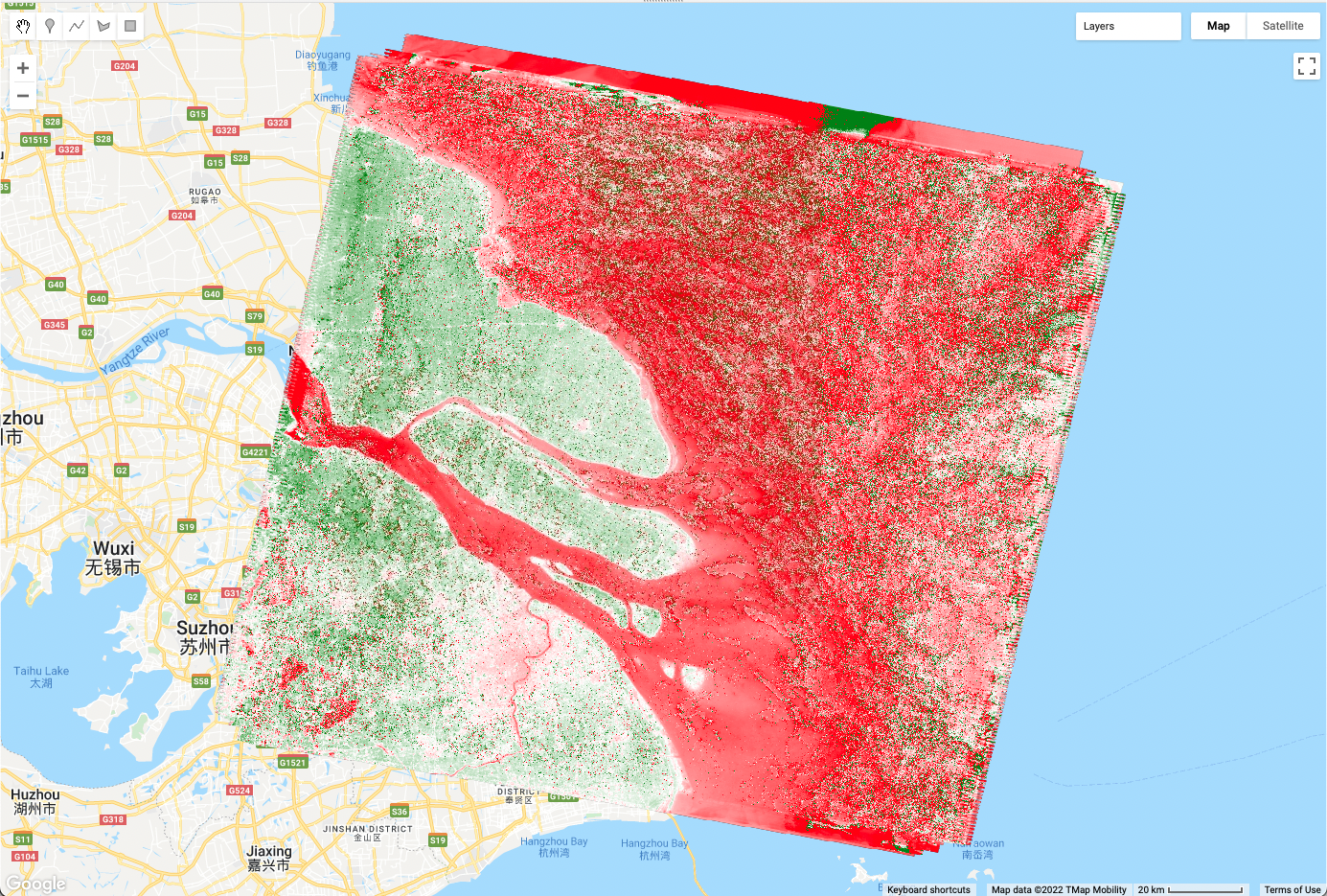
var L5EVImedian=L5EVIimages.reduce(ee.Reducer.median()); |
Fig. 4.0.2 The effects of two reducers on mapped EVI values in a filtered ImageCollection: mean image (above), and median image (below) |
There are many more reducers that work with an ImageCollection to produce a wide range of summary statistics. Reducers are not limited to returning only one item from the reduction. The minMax reducer, for example, returns a two-band image for each band it is given, one for the minimum and one for the maximum.
The reducers described here treat each pixel independently. In subsequent chapters in Part F4, you will see other kinds of reducers—for example, ones that summarize the characteristics in the neighborhood surrounding each pixel.
Code Checkpoint F40c. The book’s repository contains a script that shows what your code should look like at this point.
Synthesis
Assignment 1. Compare the mean and median images produced in Sect. 3 (Fig. 4.0.2). In what ways do they look different, and in what ways do they look alike? To understand how they work, pick a pixel and inspect the EVI values computed. In your opinion, which is a better representative of the data set?
Assignment 2. Adjust the filters to filter a different proportion of clouds, or a different date range. What effects do these changes have on the number of images and the look of the reductions made from them?
Assignment 3. Explore the ee.Filter options in the API documentation, and select a different filter that might be of interest. Filter images using it, and comment on the number of images and the reductions made from them.
Assignment 4. Change the EVI function so that it returns the original image with the EVI band appended by replacing the return statement with this: return (oneL5Image.addBands(landsat5EVI))
What does the median reducer return in that case? Some EVI values are 0. What are the conditions in which this occurs?
Assignment 5. Choose a date and location that is important to you (e.g., your birthday and your place of birth). Filter Landsat imagery to get all the low-cloud imagery at your location within 6 months of the date. Then, reduce the ImageCollection to find the median EVI. Describe the image and how representative of the full range of values it is, in your opinion.
Conclusion
In this chapter, you learned about the paradigm of filter, map, reduce. You learned how to use these tools to sift through, operate on, and summarize a large set of images to suit your purposes. Using the Filter functionality, you learned how to take a large ImageCollection and filter away images that do not meet your criteria, retaining only those images that match a given set of characteristics. Using the Map functionality, you learned how to apply a function to each image in an ImageCollection, treating each image one at a time and executing a requested set of operations on each. Using the Reduce functionality, you learned how to summarize the elements of an ImageCollection, extracting summary values of interest. In the subsequent chapters of Part 4, you will encounter these concepts repeatedly, manipulating image collections according to your project needs using the building blocks seen here. By building on what you have done in this chapter, you will grow in your ability to do sophisticated projects in Earth Engine.
Feedback
To review this chapter and make suggestions or note any problems, please go now to bit.ly/EEFA-review. You can find summary statistics from past reviews at bit.ly/EEFA-reviews-stats.
References
Cloud-Based Remote Sensing with Google Earth Engine. (n.d.). CLOUD-BASED REMOTE SENSING WITH GOOGLE EARTH ENGINE. https://www.eefabook.org/
Cloud-Based Remote Sensing with Google Earth Engine. (2024). In Springer eBooks. https://doi.org/10.1007/978-3-031-26588-4