Cloud-Based Remote Sensing with Google Earth Engine

Fundamentals and Applications

Part A2: Aquatic and Hydrological Applications

Earth Engine’s global scope and long time series allow analysts to understand the water cycle in new and unique ways. These include surface water in the form of floods and river characteristics, long-term issues of water balance, and the detection of subsurface ground water.

Chapter A2.1: Groundwater Monitoring with GRACE

Authors

A.J. Purdy, J.S. Famiglietti

Overview

The following tutorial details how to use observations from the Gravity Recovery and Climate Experiment (GRACE) to evaluate changes in groundwater storage for a large river basin. Here, you will learn how to apply remote sensing estimates of total water storage anomalies, land surface model output, and in situ observations to resolve groundwater storage changes in California’s Central Valley. The following method has been applied to study water storage changes around the world, and can be ported to quantify groundwater storage change for major river basins.  

Learning Outcomes

• Plotting changes in total water storage using GRACE.
• Mapping trends in water storage.
• Resolving changes in groundwater storage for a river basin.
• Import image collections and create image collections from assets.
• Create charts by reducing an ImageCollection with a feature geometry.

Helps if you know how to:

• Use expressions to perform calculations on image bands (Chap. F3.1).
• Write a function and map it over an ImageCollection (Chap. F4.0).
• Fit linear and nonlinear functions with regression in an ImageCollection time series (Chap. F4.6).
• Use ee.Join to join one ImageCollection to another to compute differences (Chap. F4.9).
• Filter a FeatureCollection to obtain a subset (Chap. F5.0, Chap. F5.1).

Github Code link for all tutorials

This code base is collection of codes that are freely available from different authors for google earth engine.

Github Source

Introduction to Theory

Since 2002, GRACE and the follow-on mission, GRACE-FO, have provided a new vantage to track changes in water resources (Tapley et al. 2004). GRACE holds the unique ability to directly track changes in total water storage anomalies (TWSa), according to the following equation:

TWSa=CANa + SWa + SMa + SWEa + GWa                                        (A2.1.1)

where CANa is canopy water storage anomaly, SWa is the surface water anomaly, SMa is the soil moisture anomaly, SWEa is the snow water equivalent anomaly, and GWa is the groundwater storage anomaly.

By utilizing supplemental observations from other remote sensing platforms and land surface models and rearranging Eq. A2.1.1, scientists have been able to resolve changes in groundwater storage within major river basins around the planet (Famiglietti et al. 2014). From Bangladesh (Purdy et al. 2019) and India (Rodell et al. 2009) to the Middle East (Voss et al. 2013) and the American Southwest (Castle et al. 2014), the problem of declining groundwater storage has emerged with varying levels of severity (Richey et al. 2015). Along with many other regions around the world, California shares an overreliance on groundwater (Famiglietti et al. 2011). This tutorial demonstrates the analytical steps to resolve groundwater storage changes using GRACE for California’s Central Valley.

Practicum

Section 1. Exploring the Study Area

Evaluating changes in hydrologic storage requires examining change within a hydrologically connected system. Watersheds and basins represent areas of land where precipitation drains to a common point. We will use already-generated basins from the Watershed Boundary Dataset (WBD) to delineate the drainage area for California’s Central Valley. The WBD includes hydrologic unit codes (HUCs) to identify connected basins within the United States.

In the following sections of code, we will load three basins by their unique four-digit HUCs and merge the basins together. To accomplish this task, we will use the ee.Filter.inList function to filter the basins variable by the 'huc4' property, extracting three to a variable basin.

Section 1.1. Map the Extent of Agriculture in the Region

To get a sense for the extent of agriculture in California, we can visualize all cultivated land in the Central Valley. This will map where the greatest need for water occurs.

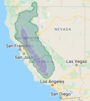
The extent of cultivated lands shows up as a translucent purple (Fig. A2.1.1).

Section 1.2. Load Reservoir Locations

California has over 150 reservoirs distributed across the state. These reservoirs vary in size and capacity and the regions of the state that they support. For the Central Valley, water conveyance infrastructure allows the transport of water from north to south. We will use our basin boundary to select the reservoirs within our basin to quantify changes in surface water storage. The list of reservoirs was gathered from the California Department of Water Resources’ Data Exchange Center (CDEC). For an application in another study region, acquiring in situ surface water storage would be required to resolve that region’s groundwater storage changes.

The blue dots that now appear on the map represent the distribution of water storage across the Central Valley. Water conveyance infrastructure and natural rivers deliver water to farms across the valley. Despite all these reservoirs, many water users continue to rely on groundwater to meet their needs. A 2011 study detailed the magnitude of this reliance using gravity-sensing satellites (Famiglietti et al. 2011). The next sections of this chapter reveal how to resolve groundwater storage changes using these methods.

Code Checkpoint A21a. The book’s repository contains a script that shows what your code should look like at this point.

Section 2. Tracking Total Water Storage Changes in California with GRACE

GRACE can directly track changes in TWSa. Changes in TWSa indicate which regions are gaining or losing water.

​​Section 2.1. Import GRACE Data and Plot Changes in Total Water Storage in California

First, we will import the image collection and select the proper band to chart.

The GRACE data imported here have already been processed to provide units of TWSa. The data contained in this dataset are units of “equivalent water thickness” anomalies. GRACE hydrologic data are presented as anomalies because GRACE does not directly observe the gravitational pull of only water. The gravity observed also includes Earth's surface (e.g., mountains). To disentangle the signal of water we can look at changes relative to a longer term mean gravity signal. The anomalies represent the difference between a given month's observation and a multi-year mean. We will now plot TWSa for basins in a large part of California (Fig. A2.1.2).

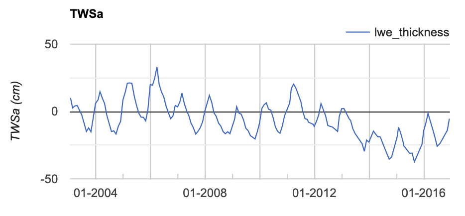
In the Console, you will see a plot of TWSa. Notice the seasonality and interannual variations in TWSa. Winter months reveal periods of maximum water storage due to snowpack, full reservoirs, and wet soil.  Summer and early fall reveal less TWSa, as the snow has melted, reservoir water has been used, and soil is drying out. Additionally, summer months are periods when groundwater is extracted and used to supplement a limited surface water supply. Evidence of drought emerged through declining TWSa between 2006–2009 and 2012–2017.

Next, we will look at the trend in TWSa for the entire period of record.

Section 2.2. Estimate the Linear Trend in TWSa Over Time

As presented in Chap. F4.6, Earth Engine can fit linear models to time series data, with unique linear fits for each pixel based on the values through time. Consider the following linear model, where et is a random error:

pt=β0 + β1t + et (1)                                                                (A2.1.2)

This is the model behind the trendline added to the chart we just created. This model is useful for detrending data and reducing non-stationarity in the time series (Shumway and Stoffer 2017). The goal of the regression is to discover the values of the β’s in each pixel.

To fit this trend model to the GRACE-based TWSa series using ordinary least squares, we can use the linearRegression reducer.

The image of coefficients, computed below, is a two-band image in which each pixel contains values for β0 and β1. The β1 value will represent the temporal slope for the GRACE mascon.

Next, we can visualize the GRACE trends to capture the spatial scales on which GRACE can resolve TWSa. GRACE is adept at capturing these changes only for larger basins.

The slope layer reveals that the Tulare Basin (the southernmost basin in the Central Valley) experienced the largest negative changes in TWSa over the time period (Fig. A2.1.3). Darker reds indicate greater negative change and blue represents positive change. This is a result of the region not receiving winter rain or snow and having the most junior surface water rights in the Central Valley.

The next steps in this chapter will review how to unpack the TWSa signal to resolve changes in groundwater storage anomalies for the basin.

Code Checkpoint A21b. The book’s repository contains a script that shows what your code should look like at this point.

Section 3. Tracking Changes in Soil Water Storage and Snow Water Equivalent in California

The Global Land Data Assimilation System (GLDAS) utilizes multiple land surface models to globally resolve fluxes in storage of water (like soil moisture and snow) and energy at a three-hour frequency (Rodell et al. 2004). An example of how to convert three-hourly GLDAS snow water equivalent to annual SWEa for 2003 can be found in script A21s1 in the book's repository. Running the supplemental script is an optional part of this lab: it is added to provide clarity on how the image assets were created for each GLDAS variable in this chapter.

For the next analysis, you will be starting with a script that imports the GLDAS SMa and SWEa processed by the methods above. GLDAS estimates of soil moisture and snow water equivalent are resolved at a three-hour temporal frequency. Therefore, we have taken the time to reduce the GLDAS data to annual means from the three-hour estimates.

Additionally, we aggregated monthly GRACE observations to annual average estimates to improve the efficiency of running this analysis. More experienced users can adapt these methods to resolve monthly changes. However, it should be noted that to replicate the same methods at a monthly cadence would require the interpolation of missing months of GRACE observations. Please use the code starting point below, as the script imports the necessary assets to complete the final analysis.

Section 3.1. Load GLDAS Soil Moisture Images from an Asset to an Image Collection

Code Checkpoint A21c. The book’s repository contains a script to use to begin this section. You will need to start with that script and paste code below into it.

When you run the script, you will see a number of assets being imported and an annual time series of GRACE. Additionally, the script is set to convert the list of annual mean soil moisture images to an ImageCollection.

Before we compute groundwater storage anomalies from GRACE and GLDAS data following Eq. A2.1.1, we should inspect the units to ensure that our math is sound. In the search bar of Earth Engine, search for “GLDAS” and click on GLDAS-2.1: Global Land Data Assimilation System, then navigate to Bands to see what the units are for 'RootMoist_inst' and 'SWE_inst'.

The units for GLDAS are currently showing as kg/m2. We need to convert the soil moisture and snow values to equivalent water depth units of centimeters. Define the following conversion variable and map this over the ImageCollection. As described in Chap. F4.0 and Chap. F4.1, mapping over an ImageCollection is similar to running a loop: You apply the same function to each image and return the value back to the ImageCollection.

In addition to converting the units, the code renames the variable and sets properties such as 'system:time_start', which is necessary in Earth Engine to plot data and compare it with other image collections. Note that you might print out the variables sm_ic and sm_ic_ts to explore the differences between them. You should notice the new band name and properties (e.g., 'system:time_start').

Next, plot the data to evaluate soil moisture anomalies during the study period.

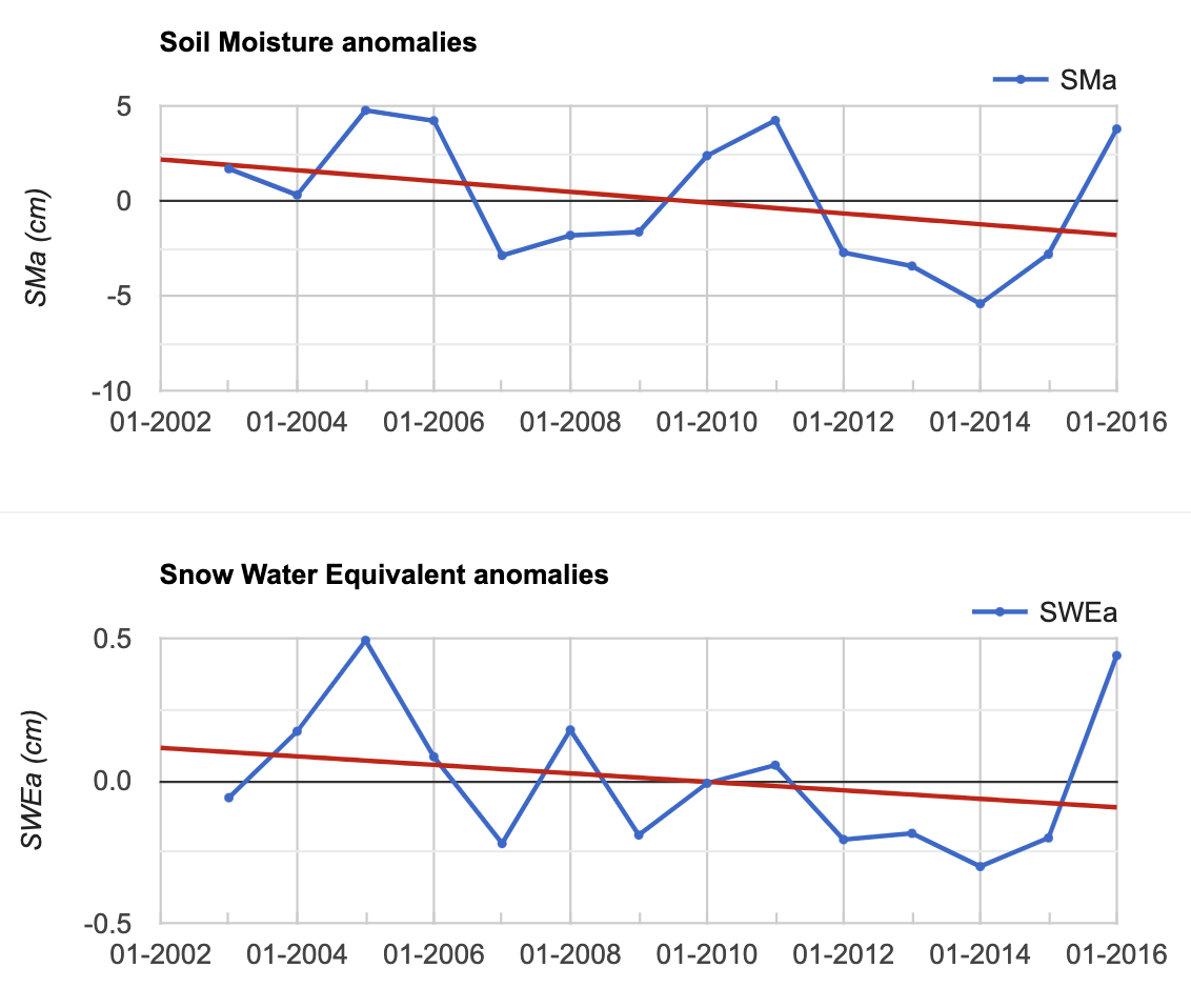
You may notice that SMa is of a similar magnitude to TWSa, but is slightly out of phase with TWSa.

Section 3.2. Load GLDAS Snow Water Equivalent Images from an Asset to an Image Collection

Use similar code to load the snow water equivalent data to Earth Engine.

Next, convert the snow values to equivalent water depth units of centimeters.

Next, we will visualize the new ImageCollection. If you did not do the previous step, your code here will not run.

You successfully plotted soil moisture and snow water equivalent (Fig. A2.1.4). You may notice that SWEa is much smaller in magnitude than the other two variables.

Code Checkpoint A21d. The book’s repository contains a script that shows what your code should look like at this point.

Section 4. Importing a Table of Surface Water Storage

Reservoir storage data from the California Data Exchange Center (CDEC) facilitated computing Surface Water storage anomalies (SWa) for the Sacramento-San Joaquin Basin. Surface water storage, unlike the other components of water storage, is not represented in land surface models. Instead, SWa is sourced from in situ observations. Here, the reservoir storage observations were summed for the Central Valley and then total converted to annual anomalies to directly compare with SWEa and SMa. Prior to reading the table of reservoir storage, we compute the area from the combined HUC8 basins.

Next, the imported table res_table is converted to an ImageCollection of constant values to facilitate combining the data with GRACE and GLDAS-resolved water storage anomalies.

Plot SWa in equivalent units of centimeters per year (Fig. A2.1.5).

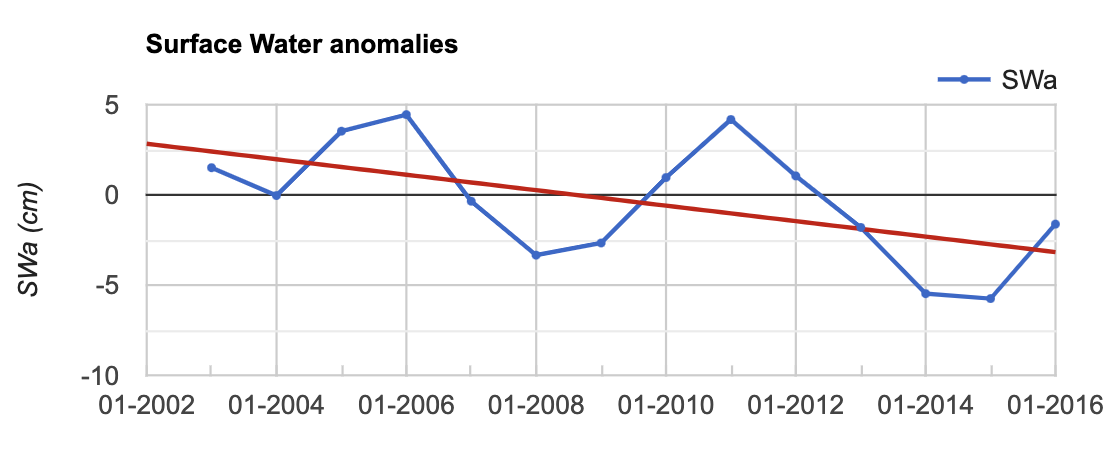
The chart shows that surface water anomalies are of a similar magnitude to soil moisture anomalies. As expected, SWa decreases during each drought period in California (2006–2008 and 2012–2016). These reservoir storage declines show use is greater than inputs during each period.

Now, we will combine the previous datasets to resolve changes in groundwater during the period of record. Unfortunately, it’s still hard to quantify change without having all the variables on one plot. It might be best to compute the differences via Eq. A2.1.1 from the introductory paragraph at the top of the document.

Code Checkpoint A21e. The book’s repository contains a script that shows what your code should look like at this point.

Section 5. Combining Image Collections

Here, you will see how to combine multiple image collections and compute differences via an expression. We will start by joining the GLDAS image collections together. This is accomplished with the ee.Join.inner function.

Next, we join the reservoir data.

Lastly, we need to repeat this step by joining GRACE to the output from the last join.

Take a moment to print out the ImageCollection GRACE_res_GLDAS.

To resolve groundwater storage changes in the basin, one can rearrange Eq. A2.1.1 to solve for GWa. Here we assume canopy storage anomalies are very small relative to other storage components and ignore them in the equation below.

GWa=TWSa - SWa - SMa - SWEa                                        (A2.1.2)

To execute this step we map an expression across an ImageCollection to produce a new variable named GWa.

You can see how the variable img is used to extract bands from the combined ImageCollection and create a new one with just one band.

We’ll plot this to see how groundwater storage is changing (Fig. A2.1.6).

You can see how reliant California is on groundwater. The chart shows large declines during recent drought periods. Using the chart, you can estimate how much groundwater was used during the 2012–2016 drought period. In the Console, hover your mouse over the chart and jot down the value for GWa in 2012 and in 2016. You will use this information, in addition to the area and unit conversion, to estimate groundwater usage during this period in cubic kilometers.

Code Checkpoint A21f. The book’s repository contains a script that shows what your code should look like at this point.

Synthesis

Assignment 1. This chapter provides a roadmap to monitor changes in groundwater storage at a basin scale using observations of TWSa from the GRACE satellites and hydrologic data from GLDAS. Now you can apply these methods to another river basin anywhere in the world.

Conclusion

In this chapter, we reviewed how GRACE observations can be used to estimate changes in water storage for a region of interest like California’s Central Valley. Specifically, this chapter demonstrated how to combine equivalent water thickness observations from GRACE with model simulations of soil moisture, snow water equivalent, and in situ reservoir storage observations to quantify groundwater storage declines. Along the way, some advanced Earth Engine skills were explored, including creating an ImageCollection from a table and joining multiple image collections. Earth Engine users now have the skills and the knowledge of GRACE observations to apply this methodology to other regions around the world.

Feedback

To review this chapter and make suggestions or note any problems, please go now to bit.ly/EEFA-review. You can find summary statistics from past reviews at bit.ly/EEFA-reviews-stats.

References

Cloud-Based Remote Sensing with Google Earth Engine. (n.d.). CLOUD-BASED REMOTE SENSING WITH GOOGLE EARTH ENGINE. https://www.eefabook.org/

Cloud-Based Remote Sensing with Google Earth Engine. (2024). In Springer eBooks. https://doi.org/10.1007/978-3-031-26588-4

Castle SL, Thomas BF, Reager JT, et al (2014) Groundwater depletion during drought threatens future water security of the Colorado River Basin. Geophys Res Lett 41:5904–5911. https://doi.org/10.1002/2014GL061055

Famiglietti JS (2014) The global groundwater crisis. Nat Clim Chang 4:945–948. https://doi.org/10.1038/nclimate2425

Famiglietti JS, Lo M, Ho SL, et al (2011) Satellites measure recent rates of groundwater depletion in California’s Central Valley. Geophys Res Lett 38 https://doi.org/10.1029/2010GL046442

Purdy AJ, David CH, Sikder MS, et al (2019) An open-source tool to facilitate the processing of GRACE observations and GLDAS outputs: An evaluation in Bangladesh. Front Environ Sci 7 https://doi.org/10.3389/fenvs.2019.00155

Richey AS, Thomas BF, Lo MH, et al (2015) Quantifying renewable groundwater stress with GRACE. Water Resour Res 51:5217–5237. https://doi.org/10.1002/2015WR017349

Rodell M, Houser PR, Jambor U, et al (2004) The global land data assimilation system. Bull Am Meteorol Soc 85:381–394. https://doi.org/10.1175/BAMS-85-3-381

Rodell M, Velicogna I, Famiglietti JS (2009) Satellite-based estimates of groundwater depletion in India. Nature 460:999–1002. https://doi.org/10.1038/nature08238

Voss KA, Famiglietti JS, Lo M, et al (2013) Groundwater depletion in the Middle East from GRACE with implications for transboundary water management in the Tigris-Euphrates-Western Iran region. Water Resour Res 49:904–914. https://doi.org/10.1002/wrcr.20078