Cloud-Based Remote Sensing with Google Earth Engine
Fundamentals and Applications

Part A2: Aquatic and Hydrological Applications
Earth Engine’s global scope and long time series allow analysts to understand the water cycle in new and unique ways. These include surface water in the form of floods and river characteristics, long-term issues of water balance, and the detection of subsurface ground water.
Chapter A2.4 River Morphology
Authors
Xiao Yang, Theodore Langhorst, Tamlin M. Pavelsky
Overview
The purpose of this chapter is to showcase Earth Engine’s application in fluvial hydrology and geomorphology. Specifically, we show examples demonstrating how to use Earth Engine to extract a river’s centerline and width, and how to calculate the bank erosion rate. At the end of this chapter, you will be able to distinguish rivers from other water bodies, perform basic morphological analyses, and detect changes in river form over time.
Learning Outcomes
- Working with Landsat surface water products.
- Calculating river centerline location and width.
- Quantifying river bank erosion.
Helps if you know how to:
- Import images and image collections, filter, and visualize (Part F1).
- Perform basic image analysis: select bands, compute indices, create masks (Part F2).
- Perform image morphological operations (Chap. F3.2).
- Write a function and map it over an ImageCollection (Chap. F4.0).
- Use reduceRegions to summarize an image with zonal statistics in irregular shapes (Chap. F5.0, Chap. F5.2).
- Work with vector data (Chap. F5.1)
Github Code link for all tutorials
This code base is collection of codes that are freely available from different authors for google earth engine.
Introduction to Theory
The shape of a river viewed from above, known as its “planview geometry,” can reveal many things about the river, including its morphological evolution and the flow of water and sediment within its channel. For example, hydraulic geometry establishes that a river’s width and its discharge satisfy a power-law relation (rating curve). Thus, one can use such a relationship to monitor a river’s discharge from river widths derived from remote sensing images (Smith et al. 1996). Similarly, in addition to the natural variability of river size, rivers also adjust their courses on the landscape as water flows from the headwaters towards lowland downstream regions. These adjustments result in meandering, lateral variations in a river’s course resulting from the erosion and accretion of sediment along the banks. Many tools have been developed to study morphological changes of rivers using remotely sensed images.
Early remote sensing of river form was done by manual interpretation of aerial imagery, but advances in computing power have facilitated and the volume of imagery from satellites has necessitated automated processing. The RivWidth software (Pavelsky and Smith 2008) first presented an automated method for river width extraction, and RivWidthCloud (RWC) (Yang et al. 2019) later applied and expanded these methods to Earth Engine. Similarly, methods for detecting changes in river form have evolved from simple tools that track hand-drawn river centerlines (Shields et al. 2000) to automated methods that can process entire basins (Constantine et al. 2014, Rowland et al. 2016). This progression towards automated software for studies in fluvial geomorphology has paired well with the capabilities of Earth Engine, and as a result many tools are being built for large-scale analysis in the cloud (Boothroyd et al. 2020).
Practicum
Section 1. Creating and Analyzing a Single River Mask
In this section, we will prepare an image and calculate some simple morphological attributes of a river. To do this, we will use a pre-classified image of surface water occurrence, identify which pixels represent the river and channel bars, and finally calculate the centerline, width, and bank characteristics.
Section 1.1. Isolate River from Water Surface Occurrence Map
Code Checkpoint A24a. The book’s repository contains a script to use to begin this section. You will need to start with that script and paste code below into it.
The script includes our example area of interest (in the variable aoi) and two helper functions for reprojecting data to the local UTM coordinates. We force this projection and scale for many of our map layers because we are trying to observe and measure the river morphology. As data is viewed at different zoom levels, the shapes and apparent connectivity of many water bodies will change. To allow a given dataset to be viewed with the same detail at multiple scales, we can force the data to be reprojected, as we do here.
The Joint Research Centre’s surface water occurrence dataset (Pekel et al. 2016) classified the entire Landsat 5, 7, and 8 history and produced annual maps that identify seasonal and permanent water classes. Here, we will include both seasonal and permanent water classes (represented by pixel values of ≥2) as water pixels (with value=1) and the rest as non-water pixels (with value=0). In this section, we will look at only one image at a time by choosing the image from the year 2000 (Fig. A2.4.1a). In the code below, bg serves as a dark background layer for other map layers to be seen easily.
// IMPORT AND VISUALIZE SURFACE WATER MASK. |
Next, we clean up the water mask by filling in small gaps by performing a closing operation (dilation followed by erosion). Areas of non-water pixels inside surface water bodies in the water mask may represent small channel bars, which we will fill in to create a simplified water mask. We identify these bars using a vectorization; however, you could do a similar operation with the connectedPixelCount method for bars up to 256 pixels in size (Fig. A2.4.1b). Filling in these small bars in the river mask improves the creation of a new centerline later in the lab.
// REMOVE NOISE AND SMALL ISLANDS TO SIMPLIFY THE TOPOLOGY. |
Note here that we forced reprojection of the map layer using the helper function rpj. This means we have to be careful to keep our domain small enough to be processed at the set scale when doing the calculation on the fly in the Code Editor; otherwise, we will run out of memory. The reprojection may not be necessary when exporting the output using a task.
In the following step, we extract water bodies in the water mask that correspond to rivers. We will define a river mask (Fig. A2.4.1d) to be pixels that are connected to the river centerline according to the filled water mask. The channel mask (Fig. A2.4.1c) is defined also by connectivity but excludes the small bars, which will give us more accurate widths and areas for change detection in Sects. 1.2 and 1.3.
We can extract the river mask by checking the water pixels’ connectivity to a provided river location database. Specifically, we use the Earth Engine method cumulativeCost to identify connectivity between the filled water mask and the pixels corresponding to the river dataset. By inverting the filled mask, the cost to traverse water pixels is 0, and the cost over land pixels is 1. Pixels in the cost map with a value of 0 are entirely connected to the Surface Water and Ocean Topography (SWOT) Mission River Database (SWORD) centerline points by water, and pixels with values greater than 0 are separated from SWORD by land. The SWORD data, which were loaded as assets in the starter script, have some points located on land, either because the channel bifurcates or because the channel has migrated, so we must exclude those from our cumulative cost parameter source, or they will appear as single pixels of 0 in our cost map.
The maxDistance parameter must be set to capture maximum distance between centerline points and river pixels. In a single-threaded river with an accurate centerline, the ideal maxDistance value would be about half the river width. However, in reality, the centerlines are not perfect, and large islands may separate pixels from their nearest centerline. Unfortunately, increasing maxDistance has a large computational penalty, so some tweaking is required to get an optimal value. We can set geodeticDistance to false to regain some computational efficiency, because we are not worried about the accuracy of the distances.
// IDENTIFYING RIVERS FROM OTHER TYPES OF WATER BODIES. |
Code Checkpoint A24b. The book’s repository contains a script that shows what your code should look like at this point.
Fig. A2.4.1 (a) water mask; (b) filled water mask with prior centerline points; (c) channel mask; (d) river mask |

Section 1.2. Obtain River Centerline and Width
After processing the image to create a river mask, we will use existing functions from RivWidthCloud to process the image further to obtain river centerlines and widths. Here we will call RivWidthCloud functions directly, taking advantage of the ability to use exposed functions from another Earth Engine script (using the require functionality to load another script as a module). We will explain the usage and purpose of the RivWidthCloud functions used here.
There are three major steps involved in obtaining river widths from a given river mask:
- Calculate one-pixel-width river centerlines.
- Estimate the direction orthogonal to the flow direction for each centerline pixel.
- Quantify river width on the channel mask along the orthogonal directions.
Extract River Centerline
We rely on morphological image analysis techniques to extract a river centerline. This process involves three steps:
- Using distance transform to enhance pixels near the centerline of the river.
- Using gradient to further isolate the centerline pixel having local minimal gradient values.
- Cleaning the raw centerline by removing spurious centerlines.
First, a distance transform is applied to the river mask, resulting in a raster image where the value of each water pixel in the river mask is replaced by the closest distance to the shore. This step is done by using the CalcDistanceMap function from RWC. From Fig. A2.4.2a, we can see that, in the distance transform, the center of the river has the highest values.
// Import existing functions from RivWidthCloud. |
Second, to isolate the centerline of the river, we apply a gradient calculation to the distance raster. If we treat the distance raster as a digital elevation model (DEM), then the locations of the river centerline can be visualized as a ridgeline. They will thus have minimal gradient value. The gradient calculation is important, as it converts a local property of the centerline (local maximum distance) to a global property (global minimal gradient) to allow extraction of the centerline with a fixed gradient threshold (Fig. A2.4.2b). We use a 0.9 threshold (recommended for RivWidth (Pavelsky and Smith, 2008) and RWC) to extract the centerline pixels from the gradient image. However, the resulting initial centerline is not always one pixel wide. To ensure a one-pixel-wide centerline, iterative image skeletonization is applied to thin the initial centerline (Fig. A2.4.2c).
// Calculate gradient of the distance raster. |
Third, the centerline from the previous step will have noise along the shoreline and will have spurious branches resulting from side channels or irregular channel forms that need to be pruned. The pruning function in RWC, CleanCenterline, works by first identifying end pixels of the centerline (i.e., centerline pixels with only one neighboring pixel) and then erasing pixels along the centerline pixels starting from the end pixels for a distance specified by MAXDISTANCE_BRANCH_REMOVAL. It will stop if the specified distance is reached or the erasing encounters a joint pixel (i.e., pixels having more than two neighboring pixels). After pruning, the final centerline should look like Fig. A2.4.2d.
// Prune the centerline to remove spurious branches. |
Fig. A2.4.2 Steps extracting river centerline: (a) distance transform of a river mask; (b) gradient of the distance map (a); (c) raw centerline after skeletonization; (d) centerline after pruning. |
Estimate Cross-Sectional Direction
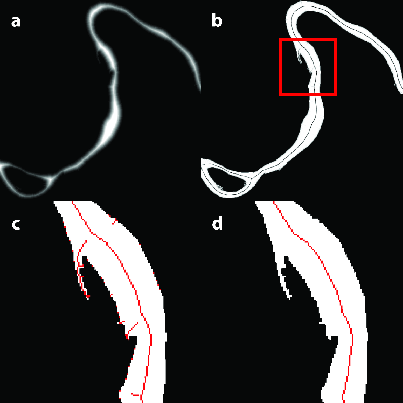
Now we will use the centerline we obtained from the previous step to help us measure the widths of the river. River width is often measured along the direction perpendicular to the flow, which we will approximate using the course of its centerline. To estimate cross-sectional directions, we convolve the centerline image with a customized kernel. The square 9 x 9 kernel has been designed so that each pixel on its rim has the radian value of the angle between the line connecting the rim pixel and the center of the kernel and the horizontal x-axis (radian angle 0). The convolution works by overlapping the center of the kernel with the centerline and calculating the average of the values of the rim pixels that overlap the centerline pixels, which corresponds to the cross-sectional direction of the particular centerline point under consideration. Here we use the function CalculateAngle to estimate the cross-sectional angles. The resulting raster will replace each centerline pixel with the value of the cross-sectional directions in degrees.
// Calculate perpendicular direction for the cleaned centerline. |
Quantify River Widths
To estimate river width, we will be using the RWC function rwGen_waterMask. This function can take any binary water mask image as input to calculate river widths, so long as the band name is ‘waterMask’ and contains the following three properties: 1) crs—UTM projection code, 2) scale—native spatial resolution, and 3) image_id—acting as an identifier for the output widths. This function works by first processing the input water mask to create all the intermediate images mentioned before (channel mask, river mask, centerline, and angle image). Then it creates a FeatureCollection of cross-sectional lines, each centered on one centerline pixel (from the centerline raster) along the direction estimated in the “Estimate Cross-Sectional Direction” section (from the angle raster) and with a length three times longer than the distance from the centerline point to the closest shoreline pixel (obtained from the distance raster). This FeatureCollection is then used in a Image.reduceRegions method as the FeatureCollection input. With a mean reducer, the result denotes the ratio between the actual river width and the length of the line segment (which is known). Thus, the final river width can be estimated by multiplying the ratio with the length of each line segment in the FeatureCollection. However, the scaling factor of 3 is chosen empirically, and can over- or underestimate the maximum extent of river width. This is because the width, scaled by 3, is the minimal distance from centerline pixels to the nearest shoreline pixels. When aligning line segments along the directions orthogonal to the river centerline, we might encounter situations when the length of these segments is too short to cover the width of the river (underestimation) or too long that they overlap with neighboring river reaches (overestimation). In both cases, the end(s) of the line segment overlaps with a pixel identified as “water” in the channel mask. Thus, additional steps are taken to flag these measurements.
The rwGen_waterMask takes four arguments—maximum search distance (unit: meter) to label river pixels, maximum size of islands (unit: pixel) to be filled in to calculate river mask, distance (unit: meter) to be pruned to clean the raw centerline, and the area of interest to carry out the width calculation. The output of the rwc function is a FeatureCollection with each feature having the properties listed in Table A2.4.1.
Table A2.4.1 Output variables from the rwc function.
longitude | Longitude of the centerline point |
latitude | Latitude of the centerline point |
width | Wetted river width measured at the centerline point |
orthogonalDirection | Angle of the cross-sectional direction at the centerline point |
flag_elevation | Mean elevation across the river surface (unit: meter) based on MERIT DEM |
image_id | Image ID of the input image |
crs | The projection of the input image |
endsInWater | Indicates inaccurate width due to the insufficient length of the cross-sectional segment that was used to measure the river width |
endsOverEdge | Indicates width too close to the edge of the image such that the width can be inaccurate |
// Estimate width. |
Section 1.3. Bank Morphology
In addition to a river’s centerline and width, we can also extract information about the banks of the river, such as their aspect and total length. To identify the banks, we simply dilate the channel mask and compare it to the original channel mask. The difference in these images represents the land pixels adjacent to the channel mask.
var bankMask=channelmask.focal_max(1).neq(channelmask); |
Next, we will calculate the aspect, or compass direction, of the bank faces. We use the Image.cumulativeCost method with the entire river channel as our source to create a new image (bankDistance) with increasing values away from the river channel, similar to an elevation map of river banks. In this image, the banks will ‘slope’ towards the river channel and we can take advantage of the terrain methods in EE. We will call the Terrain.aspect method on the bank distance and select the bank pixels by applying the bank mask. In the end, our bank aspect data will give us the direction from each bank pixel towards the center of the channel. These data could be useful for interpreting any directional preferences in erosion as a result of geological features or thawed permafrost soils from solar radiation.
var bankDistance=channelmask.not().cumulativeCost({ |
Last, we calculate the length represented by each bank pixel by convolving the bank mask with a Euclidean distance kernel. Sections of bank oriented along the pixel edges will have a value of 30 m per pixel, whereas a diagonal section will have a value of  * 30 m per pixel.
var distanceKernel=ee.Kernel.euclidean({ |
Code Checkpoint A24c. The book’s repository contains a script that shows what your code should look like at this point.
Section 2. Multitemporal River Width
Refresh the Code Editor to begin with a new script for this section.
In Sect. 1.2, we walked through the process of extracting the river centerline and width from a given water mask. In that section, we intentionally unpacked the different steps used to extract river centerline and width so that readers can: (1) get an intuitive idea of how the image processes work step by step and see the resulting images at each stage; (2) combine these functions to answer different questions (e.g., readers might only be interested in river centerlines instead of getting all the way to widths). In this section, we will walk you through how to use some high-level functions in RivWidthCloud to more efficiently implement these steps across multiple water mask images to extract time series of widths at a given location. To do this, we need to provide two inputs: a point of interest (longitude, latitude) and a collection of binary water masks. The code below re-introduces a helper function to convert between projections, then accesses other data and functionality.
var getUTMProj=function(lon, lat){ |
Remember that the widths from Sect. 1.2 are stored in a FeatureCollection with multiple width values from different locations along a centerline. To extract the multitemporal river width for a particular location along a river, we only need one width measurement from each water mask. Here, we choose the width for the centerline pixel that is nearest to the given point of interest using the function getNearestCl. This function takes the width FeatureCollection from Sect. 1.2 as input and returns a feature corresponding to the width closest to the point of interest.
// Function to identify the nearest river width to a given location. |
Then we will need to use the map method on the input collection of water masks to apply the rwc to all the water mask images. This will result in a FeatureCollection, each feature of which will contain the width quantified from one image (or time stamp).
// Multitemporal width extraction. |
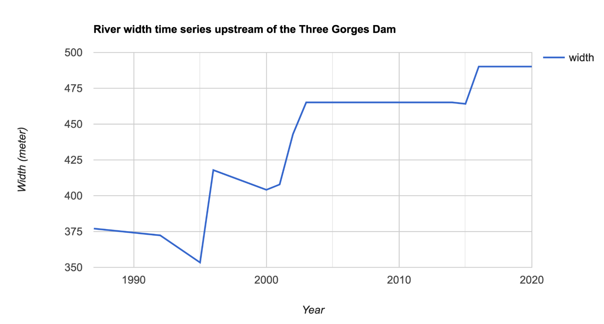
Fig. A2.4.3 River width time series upstream of the Three Gorges Dam in China. The series shows the abrupt increase in river width around the year 2003, when the dam was completed. |
Code Checkpoint A24d. The book’s repository contains a script that shows what your code should look like at this point.
Section 3. Riverbank Erosion
In this section, we will apply the methods we developed in Sect. 1 to multiple images, calculate the amount of bank erosion, and summarize our results back onto our centerline. Before doing so, we will create a new script that wraps the masking and morphology code in Sects. 1.1 and 1.3 into a function called makeChannelmask that has one argument for the year. We return an image with bands for all of the masks and bank calculations, plus a property named 'year’ that contains the year argument. If you have time, you could try to create this function on your own and then compare with our implementation of it, in the next code checkpoint. Note that we would not expect that your code would look the same, but it should ideally have the same functionality.
Code Checkpoint A24e. The book’s repository contains a script to use to begin this section. You will need to start with that script and paste code below into it.
Change Detection
We will use a section of the Madre de Dios River as our study area for this example because it migrates very quickly, more than 30 m per year in some locations. Our methods will work best if the two channel masks partially overlap everywhere along the length of the river; if there is a gap between the two masks, we will underestimate the amount of change and not be able to calculate the direction of change. As such, we will pick the years 2015 and 2020 for our example. However, in other locations, you may want to increase the time span in order to observe more change. We first create these two sets of channel masks and add them to the map (Fig. A2.4.4a).
var masks1=makeChannelmask(2015); |
Fig. A2.4.4 A single meander bend of the Madre de Dios River in Bolivia, showing areas of erosion and accretion: (a) channel mask from 2015 in blue and channel mask from 2020 in red at 50% transparency; (b) pixels that represent erosion between 2015 and 2020 |

Next, we create an image to represent the eroded area (Fig. A2.4.4b). We can quickly calculate this by comparing the channel mask in year 2 to the inverse water mask from year 1. In alluvial river systems, avulsions and meander cutoffs can leave fragments of old channels near the river. If the river meanders back into these water bodies, we want to be careful not to count these as fully eroded, which is why we need to compare our river pixels in year 2 (channel mask) to the land pixels in year 1 (inverse water mask). If you were to compare only the channel masks from year to year, water in the floodplains that is captured by the channel migration would be falsely counted as erosion.
// Pixels that are now the river channel but were previously land. |
Now we are going to approximate the direction of erosion. We will define the direction of erosion by the shortest path through the eroded area from each bank pixel in year 1 to any of the bank pixels in year 2. In reality, meandering rivers often translate their shape downvalley, which breaks our definition of the shortest path between banks. However, the shortest path produces a reasonable approximation in most cases and is easy to calculate. We will again use Image.cumulativeCost to measure the distance using the erosion image as our cost surface. The erosion image has to be dilated by 1 pixel to compensate for the missing edge pixels in the gradient calculations, and masked in order to limit the cost paths to within the eroded area.
// Erosion distance assuming the shortest distance between banks. |
Now we can use the same Terrain.aspect method that we used for the bank aspect to calculate the direction of the shortest path along our cost surface. You could also calculate this direction (and the bank aspect in Sect. 1.3) using the Image.gradient method and then calculating the tangent of the resulting x and y components.
// Direction of the erosion following slope of distance. |
Connecting to the Centerline
We now have all of our change metrics calculated as images in Earth Engine. We could export these and make maps and figures using these data. However, when analyzing a lot of river data, we often want to look at long profiles of a river or tributary networks in a watershed. In order to do this, we will use reducers to summarize our raster data back onto our vector centerline. The first step is to identify which pixels should be assigned to which centerline points. We will start by calculating a single image representing the distance to any SWORD centerline point with the FeatureCollection.distance method. Next, we will use a convolution with the Laplacian kernel (Chap. F3.2) as an edge detection method on our distance raster. By convolving the distance to the nearest SWORD node with the Laplacian kernel, we are calculating the second derivative of distance, and can find the locations where the distance surface starts sloping towards another SWORD point.
// Distance to nearest SWORD centerline point. |
Next, we need to create an image where each pixel’s value is set to the unique node identifier of the nearest SWORD centerline point. We will create a two-band image, where the first band is the concavity boundaries found in the last step, and the second band has the unique node identifiers painted on their location. When we reduce this image using the Image.reduceConnectedComponents method, we set all pixels in each region with the corresponding node ID. Last, we need to dilate these pixels to fill in the boundary gaps using a call to the Image.focalMode method.
// Reduce the pixels according to the concavity boundaries, |
Fig. A2.4.5 A section of the Madre de Dios River where each pixel is assigned to its closest centerline node |

Summarizing the Data
The final step in this section is to apply a reducer that uses our nodePixels image from the previous step to group our raster data. We will combine the reducer.forEach and reducer.group methods into our own custom function that we can use with different reducers to get our final results. The reducer.forEach method sets up a different reducer and output for each band in our image, which is necessary when we use the reducer.group method. The reducer.group method is conceptually similar to reducer.reduceRegions, except our regions are defined by an image band instead of by polygons. In some cases the group method is much faster than the reducer.reduceRegions method, particularly if you were to have to convert your regions to polygons in order to provide the input to reducer.reduceRegions. The grouped reducers in our function return a list of dictionaries. However, it is much easier to work with feature collections, so we will map over the list and create a FeatureCollection before returning from the function.
// Set up a custom reducing function to summarize the data. |
For some variables—such as the erosion, the channel mask, or the bank length—we want the total number of pixels or bank length, so we will use the Reducer.sum method with our grouped reducer function. For our aspect and directional variables, we need to use the Reducer.circularMean method to find the mean direction. The returned variables sumStats and angleStats are feature collections with properties for our reduced data and the corresponding node ID.
var dataMask=masks1.addBands(masks2).reduce(ee.Reducer |
Finally, we will join these two new feature collections to our original centerline data and print the results (Fig. A2.4.6).
var vectorData=sword.filterBounds(aoi).map(function(feat){ |
Code Checkpoint A24f. The book’s repository contains a script that shows what your code should look like at this point.
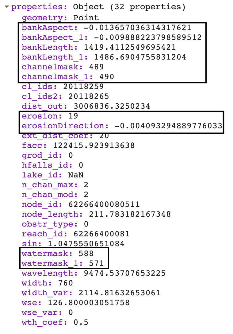
Fig. A2.4.6 The updated list of properties in our centerline dataset; new properties are outlined in black. The erosion and mask fields are in units of pixels, but you could convert to area using the Image.pixelArea method on the masks. |
This workflow can be used to add many new properties to the river centerlines based on raster calculations. For example, we calculated the amount of erosion between these two years, but you could use very similar code to calculate the amount of accretion that occurred. Other interesting properties of the river, like the slope of the banks from a DEM, could be calculated and added to our centerline dataset.
Synthesis
Assignment 1. RivWidthCloud can estimate individual channel width in the case of multichannel rivers. Change the AOI to a multichannel river and observe the resulting centerline and width data. Note down things you think are different from the single-channel case.
Assignment 2. Answer the following question. When rivers experience both variable width over time and bank migration, how can we apply the methods in this chapter to distinguish these two types of changes?
Conclusion
In this chapter, we provide ways in which Earth Engine can be used to aid river planview morphological studies. In the first half of the chapter, we show how to distinguish river pixels from other types of water bodies, as well as how to extract river centerline, river width, bank aspect, and length. In the second half of the chapter, we give examples of how to apply these methods to multitemporal image collections to estimate changes in river widths for rivers that have stable channels, and to estimate bank erosion for rivers that tend to meander quickly. The analysis makes use of both raster- and vector-based methods provided by Earth Engine to help quantify river morphology. More importantly, these methods can be applied at scale.
Feedback
To review this chapter and make suggestions or note any problems, please go now to bit.ly/EEFA-review. You can find summary statistics from past reviews at bit.ly/EEFA-reviews-stats.
References
Cloud-Based Remote Sensing with Google Earth Engine. (n.d.). CLOUD-BASED REMOTE SENSING WITH GOOGLE EARTH ENGINE. https://www.eefabook.org/
Cloud-Based Remote Sensing with Google Earth Engine. (2024). In Springer eBooks. https://doi.org/10.1007/978-3-031-26588-4
Boothroyd RJ, Williams RD, Hoey TB, et al (2021) Applications of Google Earth Engine in fluvial geomorphology for detecting river channel change. Wiley Interdiscip Rev Water 8:e21496. https://doi.org/10.1002/wat2.1496
Constantine JA, Dunne T, Ahmed J, et al (2014) Sediment supply as a driver of river meandering and floodplain evolution in the Amazon Basin. Nat Geosci 7:899–903. https://doi.org/10.1038/ngeo2282
Pavelsky TM, Smith LC (2008) RivWidth: A software tool for the calculation of river widths from remotely sensed imagery. IEEE Geosci Remote Sens Lett 5:70–73. https://doi.org/10.1109/LGRS.2007.908305
Pekel JF, Cottam A, Gorelick N, Belward AS (2016) High-resolution mapping of global surface water and its long-term changes. Nature 540:418–422. https://doi.org/10.1038/nature20584
Rowland JC, Shelef E, Pope PA, et al (2016) A morphology independent methodology for quantifying planview river change and characteristics from remotely sensed imagery. Remote Sens Environ 184:212–228. https://doi.org/10.1016/j.rse.2016.07.005
Shields Jr FD, Simon A, Steffen LJ (2000) Reservoir effects on downstream river channel migration. Environ Conserv 27:54–66. https://doi.org/10.1017/S0376892900000072
Smith LC, Isacks BL, Bloom AL, Murray AB (1996) Estimation of discharge from three braided rivers using synthetic aperture radar satellite imagery: Potential application to ungaged basins. Water Resour Res 32:2021–2034. https://doi.org/10.1029/96WR00752
Yang X, Pavelsky TM, Allen GH, Donchyts G (2020) RivWidthCloud: An automated Google Earth Engine algorithm for river width extraction from remotely sensed imagery. IEEE Geosci Remote Sens Lett 17:217–221. https://doi.org/10.1109/LGRS.2019.2920225