Cloud-Based Remote Sensing with Google Earth Engine

Fundamentals and Applications

Part A3: Terrestrial Applications

Earth’s terrestrial surface is analyzed regularly by satellites, in search of both change and stability. These are of great interest to a wide cross-section of Earth Engine users, and projects across large areas illustrate both the challenges and opportunities for life on Earth. Chapters in this Part illustrate the use of Earth Engine for disturbance, understanding long-term changes of rangelands, and creating optimum study sites.

Chapter A3.1: Active fire monitoring

Authors

Morgan A. Crowley* and Tianjia Liu* (*shared first-authorship)

Overview

Fire monitoring across the world benefits from raw satellite imagery and processed fire-mapping datasets. Google Earth Engine supports fire monitoring throughout fire seasons with satellite data from sources like Landsat 8, Sentinel-2, and Moderate Resolution Imaging Spectroradiometer (MODIS), and by hosting multiple fire datasets from the Geostationary Operational Environmental Satellite (GOES) and the Fire Information for Resource Management System (FIRMS). In this chapter, you will access, process, and explore three fire monitoring datasets available in the data catalog. By the end of this chapter, you will learn how to use the Code Editor and user apps to summarize and compare the characteristics of fires, fire seasons, and fire-monitoring datasets.

Learning Outcomes

• Accessing and visualizing fire-monitoring datasets in the JavaScript UI.
• Adjusting previously drafted code to calculate fire characteristics in the JavaScript UI for a fire of your choice.
• Exploring fire metrics and visualization with user apps.
• Identifying pros and cons of different fire datasets for a variety of monitoring objectives.

Helps if you know how to:

• Import images and image collections, filter, and visualize (Part F1).
• Write a function and map it over an ImageCollection (Chap. F4.0).
• Filter a FeatureCollection to obtain a subset (Chap. F5.0, Chap. F5.1).
• Design user interfaces for an Earth Engine App (Chap. F6.3).
• Access and interact with previously made Earth Engine user apps (Chap. F6.3).

Github Code link for all tutorials

This code base is collection of codes that are freely available from different authors for google earth engine.

Github Source

Introduction to Theory

Fire has many roles around the world. It is both a naturally occurring ecological process in fire-prone regions and a tool used by humans for land and resource management. However, fires and their emissions continue to have more extreme impacts as human settlements expand, climatic conditions become less predictable, and fire seasons lengthen (Jolly et al. 2015). To better identify and quantify the effects of fires across the globe, it is vital to monitor fires using various methods, including hand-drawn maps, ground-based sensors, GPS tracking, aerial surveys, imagery collection, and satellite-based data (Andela et al. 2019; Archibald et al. 2009; Nogueira et al. 2016; Stinson et al. 2011; Veraverbeke et al. 2014).

Different sources of satellite imagery can be used to visualize fire conditions and progressions, calculate band ratios reflecting disturbance and fire severity, and map burned areas with training data-informed classification algorithms (Crowley et al. 2019a; Crowley et al. 2019b; Hawbaker et al. 2017; Hermosilla et al. 2018; Parks 2014; Parks et al. 2019; Veraverbeke et al. 2014). Many premade fire datasets are readily available for monitoring global fire locations, extents, and progressions (Andela et al. 2019; Chuvieco et al. 2016; Giglio et al. 2016; Humber et al. 2018). In the case of existing fire datasets available for large spatial and temporal extents, remote sensing scientists apply their robust classification algorithms on satellite imagery and other geospatial data. Earth Engine makes fire monitoring more accessible by sharing multiple data sources in the data catalog so users can easily access and process these data to meet their desired objectives (Liu and Crowley 2021).

Practicum

Section 1. Fire Datasets in Google Earth Engine

In the following example, we use MODIS and GOES datasets (Table A3.1.1) to map the Bobcat Fire, a megafire that burned 115,796 acres in Los Angeles County, California, in September 2020.

Table A3.1.1        MODIS and GOES fire mapping datasets available in the Google Earth Engine data catalog

* MODIS Terra (from 2000), MODIS Aqua (from 2002), GOES-16 (from 2016), GOES-17 (from 2017)

** Can be disaggregated into daily resolution using the MCD64A1 burn date variable

First, we need to define temporal and spatial variables to filter the datasets, namely the approximate ignition coordinates and start date of the fire.

Using the ignition date (September 6, 2020), we can define separate date ranges to filter the active fire and burned area datasets to account for differences in the temporal structure of the datasets—i.e., daily versus monthly. Here we set the temporal filter range for active fire datasets as the two-week period starting from the ignition date and for the burned area dataset as the month of September. The duration variables can be modified according to the fire of interest.

With these input variables defined, we can preprocess the fire datasets. We will upload a high-resolution reference perimeter provided by the U.S. National Interagency Fire Center (NIFC) and then add the MODIS and GOES datasets from the Earth Engine data catalog.

Reference Fire Perimeter 

The NIFC produces wildland fire perimeters using information from local fire agencies. For this tutorial, we uploaded the NIFC perimeter for the Bobcat Fire, converting it from a shapefile to an Earth Engine asset. We will access the asset from the book repository and use it as a reference layer to compare with the MODIS and GOES datasets.

MODIS Active Fire Products

The gridded 1 km MODIS active fire datasets, MOD14A1 (Terra) and MYD14A1 (Aqua), have daily collection rates and global coverage (Giglio et al. 2016; Giglio 2010). The MODIS sensor is mounted on the two separate satellites, Terra and Aqua, both operated by NASA for environmental monitoring. Here we define two functions to process the fire mask and fire radiative power (FRP) variables. The fire mask provides a categorical classification of the confidence in fire detection, where values ≥7 indicate that fire is present. FRP is a continuous variable that is a proxy for fire intensity, in units of megawatts (MW). Note that MODIS FRP must be multiplied by 0.1 to be in units of MW.

MODIS Burned Area Product

The gridded 500 m MODIS burned area dataset, MCD64A1, is monthly with global coverage but can be disaggregated to daily resolution with its burn date variable (Giglio et al. 2016; Humber et al. 2018). Here we define a function to retrieve the burn date.

GOES Active Fire Products        

The gridded 2 km GOES-16 (East) and GOES-17 (West) active fire datasets cover North and South America in the full disk version (FDCF) with a temporal revisit rate of 15-minute increments (Hall et al. 2019; Schroeder et al. 2008). The two GOES satellites are operated by the National Oceanic and Atmospheric Administration (NOAA) and are primarily used for meteorological monitoring. Note that the pixel orientation and shape differ between GOES-16 and GOES-17 because of the different viewing angles of the two satellites.

Now, we will visualize the three datasets, along with the reference Bobcat Fire perimeter, and plot the layers on the Earth Engine interactive map.

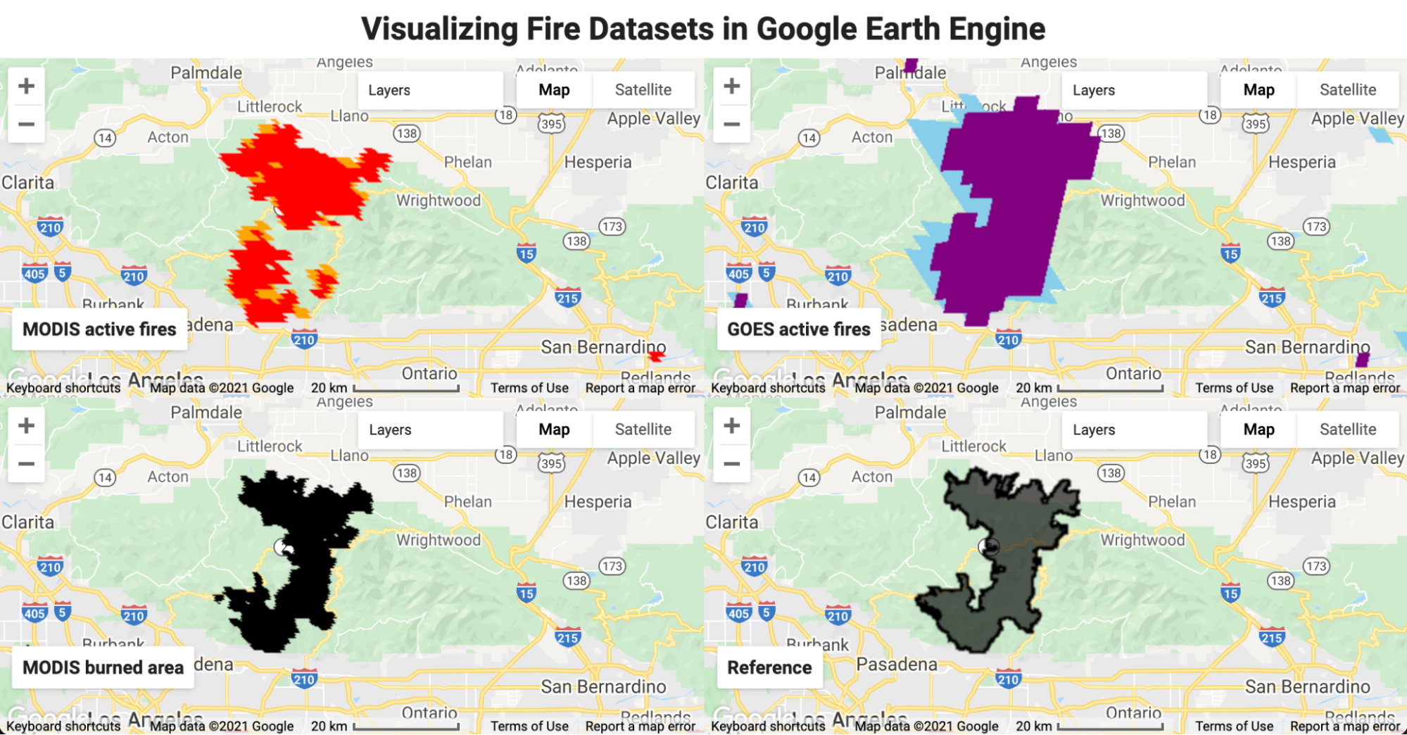
We can also visualize the datasets side by side as shown in Fig. A3.1.1 by using the ui.Panel and ui.Map.Linker using the code provided by the “Linked Maps” script under Examples > User Interface in the Scripts panel.

Code Checkpoint A31a. The book’s repository contains a script that shows what your code should look like at this point.

Question 1. How does the burned area classification (i.e., burned versus unburned) and the spatial resolution (i.e., pixel size) differ across the three datasets?

Question 2. There appears to be a gap in fire activity between the MODIS incident data and burned area map for the Bobcat Fire, as shown in the split-panel app. What differences in the datasets might account for the mismatched fire classifications?                 Hint: Use https://worldview.earthdata.nasa.gov/ to examine raw MODIS imagery of the fire location and date.

Question 3. How does the temporal resolution of 15 minutes for GOES impact monitoring fires in the event of smoke and haze?

Section 2. In-Depth Visualization and Analysis of Fires in Earth Engine Apps

Earth Engine Apps help to curate in-depth visualization and analysis of fires. Here we present two apps using datasets from the Earth Engine public data catalog.

In the remainder of this chapter, you will use these two apps to learn more about the Bobcat Fire and to explore findings from the two datasets.

App 1: FIRMS Active Fires

FIRMS currently monitors active fires detected by MODIS, Visible Infrared Imaging Radiometer Suite (VIIRS), and NOAA-20 in near-real time. FIRMS retains the coordinates of the centroid of pixels where one or more active fires are detected. The FIRMS dataset in the Earth Engine data catalog includes only MODIS active fires, gridded at 1 km spatial resolution. Note that the FIRMS dataset is meant for exploratory rather than rigorous scientific analyses.

The “FIRMS Active Fires” Earth Engine app allows users to visualize the spatial and temporal variation in FIRMS active fires within a defined region.

Code Checkpoint A31b. The book’s repository contains information about accessing the app.

Using the control panel, you can specify the date range (start year, end year, and day-of-year range) and draw a region of interest using either a rectangle or a polygon. The map shows the number of years that one or more active fires were detected in each pixel. The chart panel shows the total daily fire counts within the region as a timeseries, where each color represents a different year (Fig. A3.1.2). You can also change the chart type to display the cumulative active fire count.

Question 4. Navigate to the Bobcat Fire using the ignition coordinates (longitude, latitude). Using the satellite or map base layer, draw a polygon similar to the one shown in a Fig. A3.1.2. Submit your task and confirm your results with the above details.

Code Checkpoint A31c. The book’s repository contains information about how your app should look at this point.

Question 5. Examine the chart. Approximately how many days did the fire actively burn? Hint: Hover over the chart and compare the first DOY value and the final DOY value.

App 2: U.S. Fire Dashboard

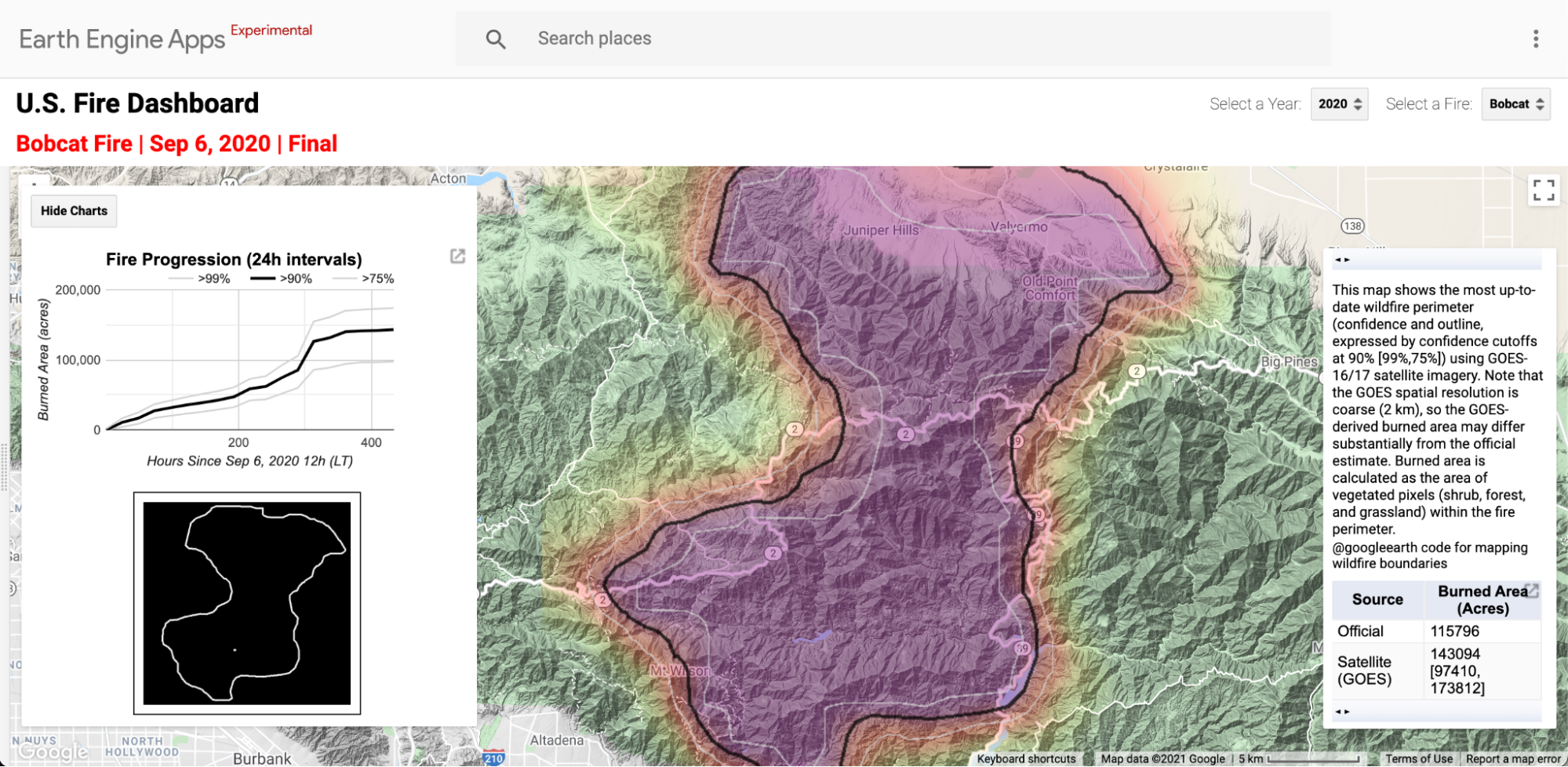
In a more advanced app, the “U.S. Fire Dashboard”, GOES-16/17 gridded active fires are used to calculate a smoothed burn perimeter for the various wildfires in 2020 by modifying the code from the Google Earth Engine Medium article, “How to generate wildfire boundary maps with Earth Engine” (Restif and Hoffman 2020). The code takes advantage of the different GOES-16 and GOES-17 pixel orientation and shape to downscale the burn classification to a finer resolution than that of the native GOES imagery. In the following example, we will use this app to visualize how the Bobcat Fire progressed in space and time from ignition (Fig. A3.1.3).

Code Checkpoint A31d. The book’s repository contains information about accessing the app.

Question 6. Navigate to the Bobcat Fire using the dropdown panel at the top right corner of the app and wait a few minutes for the results to load. Examine the fire progression chart drawn at the top of the left panel. How many hours did it take for the fire to reach its maximum burned area? Now examine the animated fire progression GIF at the bottom of the left panel. What direction did the Bobcat Fire burn?

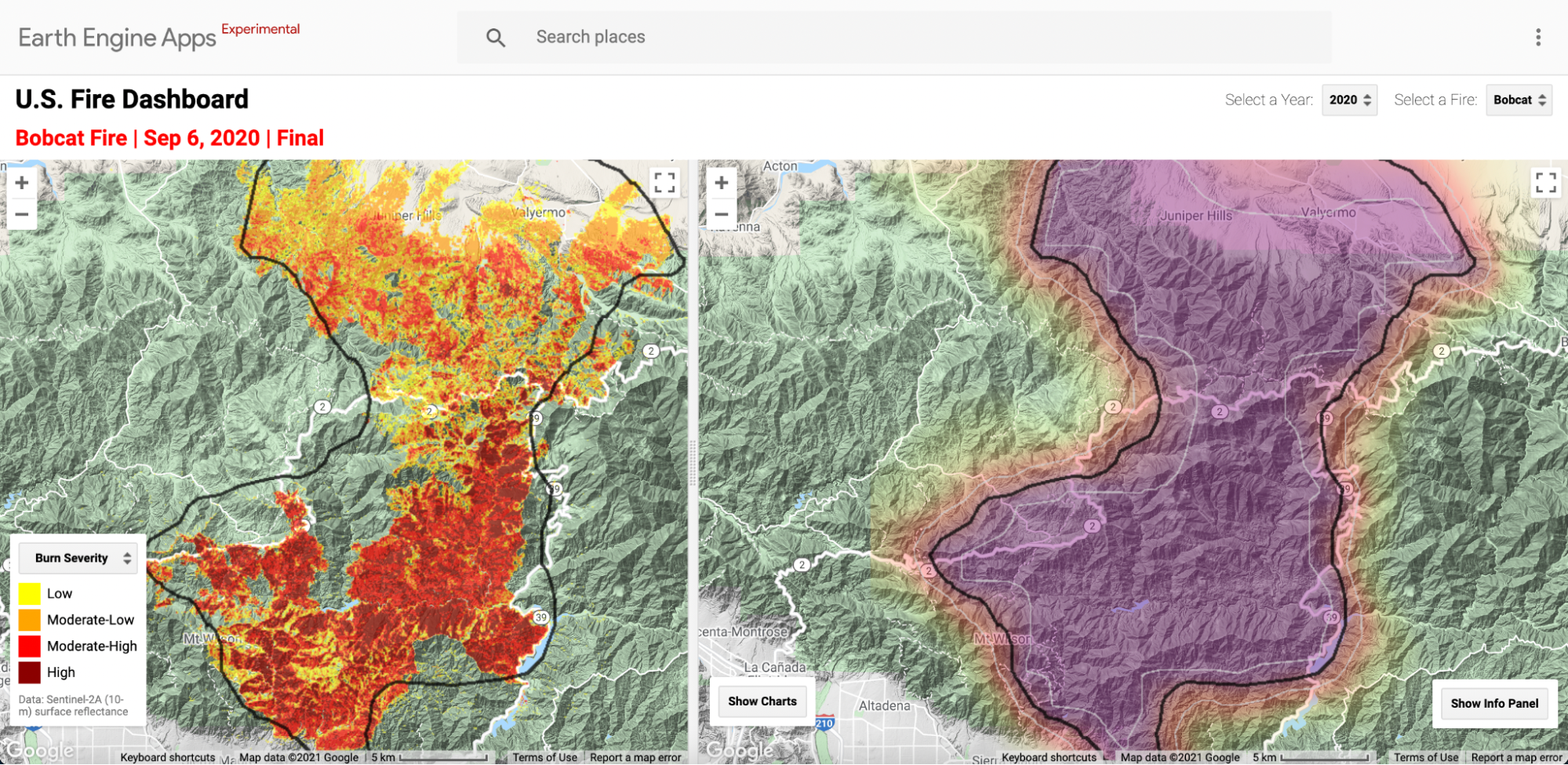
Question 7. Now drag the split panel from the left to reveal a second panel. Use the dropdown menu on the legend to navigate to the burn severity option. Let the results load and you will see a burn severity map calculated from Sentinel-2 imagery in the left-hand panel. For this question, consider all burn severities as burned area. Where do the Sentinel-2 map and the GOES map for the Bobcat Fire agree on the burned area (Fig. A3.1.4)? Where do they disagree?

Question 8. Having explored the different datasets and the two apps, what features would you include in your own wildfire mapping app? Explore additional data sources in the Synthesis section to get more inspiration for your app.

Synthesis

Assignment 1. You are now familiar with three fire datasets available in Earth Engine. Table A3.1.2 presents some additional fire datasets that are also available in the data catalog. Use the example codes written in each dataset’s description in the data catalog to load and explore the datasets in the Code Editor.

Table A3.1.2        Additional external fire mapping datasets that can be uploaded into Google Earth Engine. For each dataset, we describe their variable type, resolution, geographic coverage, and temporal extent features.

Assignment 2. While Earth Engine provides access to many existing fire datasets, there are other commonly used fire mapping datasets that are also quite useful for examining active and past fires. Select and import one of the external fire datasets shown in Table A3.1.3 into Earth Engine as a personal asset to compare it with the active fire datasets already loaded in your script.

Table A3.1.3 Additional external fire-related datasets that can be uploaded into Google Earth Engine. For each dataset, we describe their variable type, resolution, geographic coverage, and temporal extent features.

Assignment 3. In addition to comparing active fire maps using the datasets suggested in Tables A3.1.2 and ​​A3.1.3, you can examine fire conditions and impacts using ancillary datasets readily available in Earth Engine. For example, you can overlay the fire datasets with vegetation conditions and fire regimes from the LANDFIRE program to better understand the ecological context of active fires.

Select one ancillary dataset to load from the data catalog and explore it alongside an active fire dataset. Land cover datasets such as MODIS, the USGS National Land Cover Database, and Copernicus Global Land Cover can help indicate types of fires and where they are occurring. By examining active fire maps with aerosol and other emission data from Sentinel-5P and MODIS Multi-Angle Implementation of Atmospheric Correction, you can begin to identify relationships between fires and air quality. These are just some of the many analyses you can explore using ancillary datasets that are already on hand in the data catalog.

Conclusion

Earth Engine provides access to multiple fire monitoring datasets that are useful for tracking active fires throughout fire seasons and retrospectively for prior years. In this chapter, you examined one fire using three datasets (MODIS active fire, MODIS burned areas, and GOES active fire). You learned how to access, visualize, and analyze the raster datasets by adjusting code in the Code Editor and interacting with the data in premade user apps. By comparing the fire mapping characteristics of each dataset, you learned how to weigh the pros and cons of existing datasets for meeting fire mapping objectives. Now that you understand the basics of what we look for in fire mapping, you can compare additional fire datasets available in Earth Engine, or explore how to make your dataset using satellite and other geospatial data.

Feedback

To review this chapter and make suggestions or note any problems, please go now to bit.ly/EEFA-review. You can find summary statistics from past reviews at bit.ly/EEFA-reviews-stats.

References

Cloud-Based Remote Sensing with Google Earth Engine. (n.d.). CLOUD-BASED REMOTE SENSING WITH GOOGLE EARTH ENGINE. https://www.eefabook.org/

Cloud-Based Remote Sensing with Google Earth Engine. (2024). In Springer eBooks. https://doi.org/10.1007/978-3-031-26588-4

Andela N, Morton DC, Giglio L, et al (2017) A human-driven decline in global burned area. Science 356:1356–1362. https://doi.org/10.1126/science.aal4108

Andela N, Morton DC, Giglio L, et al (2019) The Global Fire Atlas of individual fire size, duration, speed and direction. Earth Syst Sci Data 11:529–552. https://doi.org/10.5194/essd-11-529-2019

Archibald S, Roy DP, van Wilgen BW, Scholes RJ (2009) What limits fire? An examination of drivers of burnt area in Southern Africa. Glob Chang Biol 15:613–630. https://doi.org/10.1111/j.1365-2486.2008.01754.x

Chuvieco E, Yue C, Heil A, et al (2016) A new global burned area product for climate assessment of fire impacts. Glob Ecol Biogeogr 25:619–629. https://doi.org/10.1111/geb.12440

Crowley MA, Cardille JA, White JC, Wulder MA (2019) Generating intra-year metrics of wildfire progression using multiple open-access satellite data streams. Remote Sens Environ 232:111295. https://doi.org/10.1016/j.rse.2019.111295

Crowley MA, Cardille JA, White JC, Wulder MA (2019) Multi-sensor, multi-scale, Bayesian data synthesis for mapping within-year wildfire progression. Remote Sens Lett 10:302–311. https://doi.org/10.1080/2150704X.2018.1536300

Giglio L (2010) MODIS collection 5 active fire product user’s guide version 2.4. Sci. Cyst. Appl. Incl. University of Maryland

Giglio L, Schroeder W, Justice CO (2016) The collection 6 MODIS active fire detection algorithm and fire products. Remote Sens Environ 178:31–41. https://doi.org/10.1016/j.rse.2016.02.054

Hall JV, Zhang R, Schroeder W, et al (2019) Validation of GOES-16 ABI and MSG SEVIRI active fire products. Int J Appl Earth Obs Geoinf 83:101928. https://doi.org/10.1016/j.jag.2019.101928

Hawbaker TJ, Vanderhoof MK, Beal YJ, et al (2017) Mapping burned areas using dense time-series of Landsat data. Remote Sens Environ 198:504–522. https://doi.org/10.1016/j.rse.2017.06.027

Hermosilla T, Wulder MA, White JC, et al (2018) Disturbance-informed annual land cover classification maps of Canada’s forested ecosystems for a 29-year Landsat time series. Can J Remote Sens 44:67–87. https://doi.org/10.1080/07038992.2018.1437719

Humber ML, Boschetti L, Giglio L, Justice CO (2019) Spatial and temporal intercomparison of four global burned area products. Int J Digit Earth 12:460–484. https://doi.org/10.1080/17538947.2018.1433727

Jolly WM, Cochrane MA, Freeborn PH, et al (2015) Climate-induced variations in global wildfire danger from 1979 to 2013. Nat Commun 6:1–11. https://doi.org/10.1038/ncomms8537

Liu T, Crowley MA (2021) Detection and impacts of tiling artifacts in MODIS burned area classification. IOP SciNotes 2:014003. https://doi.org/10.1088/2633-1357/abd8e2

Nogueira JMP, Ruffault J, Chuvieco E, Mouillot F (2017) Can we go beyond burned area in the assessment of global remote sensing products with fire patch metrics? Remote Sens 9:7. https://doi.org/10.3390/rs9010007

Parks SA (2014) Mapping day-of-burning with coarse-resolution satellite fire-detection data. Int J Wildl Fire 23:215–223. https://doi.org/10.1071/WF13138

Parks SA, Holsinger LM, Koontz MJ, et al (2019) Giving ecological meaning to satellite-derived fire severity metrics across North American forests. Remote Sens 11:1735. https://doi.org/10.3390/rs11141735

Restif BC, Hoffman A, Engineers SS, Response C (2020) How to generate wildfire boundary maps with Earth Engine. In: Google Earth and Earth Engine. https://medium.com/google-earth/how-to-generate-wildfire-boundary-maps-with-earth-engine-b38eadc97a38. Accessed 1 Oct 2020

Schroeder W, Prins E, Giglio L, et al (2008) Validation of GOES and MODIS active fire detection products using ASTER and ETM+ data. Remote Sens Environ 112:2711–2726. https://doi.org/10.1016/j.rse.2008.01.005

Stinson G, Kurz WA, Smyth CE, et al (2011) An inventory-based analysis of Canada’s managed forest carbon dynamics, 1990 to 2008. Glob Chang Biol 17:2227–2244. https://doi.org/10.1111/j.1365-2486.2010.02369.x

Veraverbeke S, Sedano F, Hook SJ, et al (2014) Mapping the daily progression of large wildland fires using MODIS active fire data. Int J Wildl Fire 23:655–667. https://doi.org/10.1071/WF13015