Cloud-Based Remote Sensing with Google Earth Engine

Fundamentals and Applications

Part F4: Interpreting Image Series

One of the paradigm-changing features of Earth Engine is the ability to access decades of imagery without the previous limitation of needing to download all the data to a local disk for processing. Because remote-sensing data files can be enormous, this used to limit many projects to viewing two or three images from different periods. With Earth Engine, users can access tens or hundreds of thousands of images to understand the status of places across decades.

Chapter F4.5: Interpreting Annual Time Series with LandTrendr

Authors

Robert Kennedy, Justin Braaten, Peter Clary

Overview

Time-series analysis of change can be achieved by fitting the entire spectral trajectory using simple statistical models. These allow us to both simplify the time series and to extract useful information about the changes occurring. In this chapter, you will get an introduction to the use of LandTrendr, one of these time-series approaches used to characterize time series of spectral values.

Learning Outcomes

• Evaluating yearly time-series spectral values to distinguish between true change and artifacts.
• Recognizing disturbance and growth signals in the time series of annual spectral values for individual pixels.
• Interpreting change segments and translating them to maps.
• Applying parameters in a graphical user interface to create disturbance maps in forests.

Assumes you know how to:

• Calculate and interpret vegetation indices (Chap. F2.0)
• Interpret bands and indices in terms of land surface characteristics (Chap. F2.0).

Github Code link for all tutorials

This code base is collection of codes that are freely available from different authors for google earth engine.

Github Source

Introduction to Theory

Land surface change happens all the time, and satellite sensors witness it. If a spectral index is chosen to match the type of change being sought, surface change can be inferred from changes in spectral index values. Over time, the progression of spectral values witnessed in each pixel tells a story of the processes of change, such as growth and disturbance. Time-series algorithms are designed to leverage many observations of spectral values over time to isolate and describe changes of interest, while ignoring uninteresting change or noise.

In this lab, we use the LandTrendr time-series algorithms to map change. The LandTrendr algorithms apply “temporal segmentation” strategies to distill a multiyear time series into sequential straight-line segments that describe the change processes occurring in each pixel. We then isolate the segment of interest in each pixel and make maps of when, how long, and how intensely each process occurred. Similar strategies can be applied to more complicated descriptions of the time series, as is seen in some of the chapters that follow this one.

Practicum

For this lab, we will use a graphical user interface (GUI) to teach the concepts of LandTrendr.

Code Checkpoint F45a. The book’s repository contains information about accessing the LandTrendr interface.

Section 1. Pixel Time Series

When working with LandTrendr for the first time in your area, there are two questions you must address.  

First, is the change of interest detectable in the spectral reflectance record? If the change you are interested in does not leave a pattern in the spectral reflectance record, then an algorithm will not be able to find it.  

Second, can you identify fitting parameters that allow the algorithm to capture that record? Time series algorithms apply rules to a temporal sequence of spectral values in a pixel, and simplify the many observations into more digestible forms, such as the linear segments we will work with using LandTrendr. The algorithms that do the simplification are often guided by parameters that control the way the algorithm does its job.

The best way to begin assessing these questions is to look at the time series of individual pixels. In Earth Engine, open and run the script that generates the GUI we have developed to easily deploy the LandTrendr algorithms. Run the script, and you should see an interface that looks like the one shown in Fig. 4.5.1.

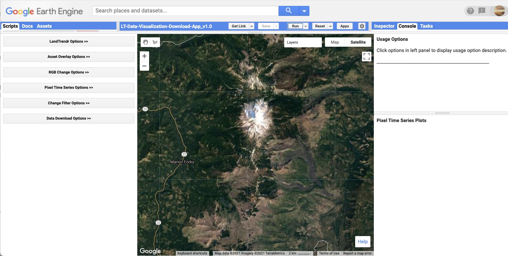
The LandTrendr GUI consists of three panels: a control panel on the left, a reporting panel on the right, and a Map panel in the center. The control panel is where all of the functionality of the interface resides. There are several modules,and each is accessed by clicking on the double arrow to the right of the title. The  Map panel defaults to a location in Oregon but can be manually moved anywhere in the world. The reporting panel shows messages about how to use functions, as well as providing graphical outputs.

Next, expand the “Pixel Time Series Options” function. For now, simply use your mouse to click somewhere on the map. Wait a few seconds even though it looks like nothing is happening – be patient!! The GUI has sent information to Earth Engine to run the LandTrendr algorithms at the location you have clicked, and is waiting for the results. Eventually you should see a chart appear in the reporting panel on the right. Fig. 4.5.2 shows what one pixel looks like in an area where the forest burned and began regrowth. Your chart will probably look different.

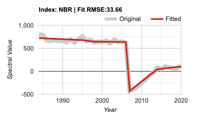
The key to success with the LandTrendr algorithm is interpreting these time series. First, let’s examine the components of the chart. The x-axis shows the year of observation. With LandTrendr, only one observation per year is used to describe the history of a pixel; later, we will cover how you control that value. The y-axis shows the spectral value of the index that is chosen. In the default mode, the Normalized Burn Ratio (as described in Chap. F4.4). Note that you also have the ability to pick more indices using the checkboxes on the control panel on the left. Note that we scale floating point (decimal) indices by 1000. Thus, an NBR value of 1.0 would be displayed as 1000.

In the chart area, the thick gray line represents the spectral values observed by the satellite for the period of the year selected for a single 30 m Landsat pixel at the location you have chosen. The red line is the output from the temporal segmentation that is the heart of the LandTrendr algorithms. The title of the chart shows the spectral index, as well as the root-mean-square error of the fit. 

To interpret the time series, first know which way is “up” and “down” for the spectral index you’re interested in. For the NBR, the index goes up in value when there is more vegetation and less soil in a pixel. It goes down when there is less vegetation. For vegetation disturbance monitoring, this is useful.

Next, translate that change into the changes of interest for the change processes you’re interested in. For conifer forest systems, the NBR is useful because it drops precipitously when a disturbance occurs, and it rises as vegetation grows.  

In the case of Fig. 4.5.2, we interpret the abrupt drop as a disturbance, and the subsequent rise of the index as regrowth or recovery (though not necessarily to the same type of vegetation).

Tip: LandTrendr is able to accept any index, and advanced users are welcome to use indices of their own design. An important consideration is knowing which direction indicates “recovery” and “disturbance” for the topic you are interested in. The algorithms favor detection of disturbance and can be controlled to constrain how quickly recovery is assumed to occur (see parameters below).  

For LandTrendr to have any hope of finding the change of interest, that change must be manifested in the gray line showing the original spectral values. If you know that some process is occurring and it is not evident in the gray line, what can you do?

One option is to change the index. Any single index is simply one view of the larger spectral space of the Landsat Thematic Mapper sensors. The change you are interested in may cause spectral change in a different direction than that captured with some indices. Try choosing different indices from the list. If you click on different checkboxes and re-submit the pixel, the fits for all of the different indices will appear.

Another option is to change the date range. LandTrendr uses one value per year, but the value that is chosen can be controlled by the user. It’s possible that the change of interest is better identified in some seasons than others. We use a medoid image compositing approach, which picks the best single observation each year from a date range of images in an ImageCollection. In the GUI, you can change the date range of imagery used for compositing in the Image Collection portion of the LandTrendr Options menu (Fig. F4.5.4).  

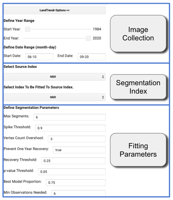
Change the Start Date and End Date to find a time of year when the distinction between cover conditions before and during the change process of interest is greatest.

There are other considerations to keep in mind. First, seasonality of vegetation, water, or snow often can affect the signal of the change of interest. And because we use an ImageCollection that spans a range of dates, it’s best to choose a date range where there is not likely to be a substantial change in vegetative state from the beginning to the end of the date range. Clouds can be a factor too. Some seasons will have more cloudiness, which can make it difficult to find good images. Often with optical sensors, we are constrained to working with periods where clouds are less prevalent, or using wide date ranges to provide many opportunities for a pixel to be cloud-free.

It is possible that no combination of index or data range is sensitive to the change of interest. If that is the case, there are two options: try using a different sensor and change detection technique, or accept that the change is not discernible. This can often occur if the change of interest occupies a small portion of a given 30 m by 30 m Landsat pixel, or if the spectral manifestation of the change is so subtle that it is not spectrally separable from non-changed pixels

Even if you as a human can identify the change of interest in the spectral trajectory of the gray line, an algorithm may not be able to similarly track it. To give the algorithm a fighting chance, you need to explore whether different fitting parameters could be used to match the red fitted line with the gray source image line.  

The overall fitting process includes steps to reduce noise and best identify the underlying signal. The temporal segmentation algorithms are controlled by fitting parameters that are described in detail in Kennedy et al. (2010). You adjust these parameters using the Fitting Parameters block of the LandTrendr Options menu. Below is a brief overview of what values are often useful, but these will likely change as you use different spectral indices.

First, the minimum observations needed criterion is used to evaluate whether a given trajectory has enough unfiltered (i.e., clear observation) years to run the fitting. We suggest leaving this at the default of 6.

The segmentation begins with a noise-dampening step to remove spikes that could be caused by unfiltered clouds or shadows. The spike threshold parameter controls the degree of filtering. A value of 1.0 corresponds to no filtering, and lower values corresponding to more severe filtering. We suggest leaving this at 0.9; if changed, a range from 0.7 to 1.0 is appropriate.

The next step is finding vertices. This begins with the start and end year as vertex years, progressively adding candidate vertex years based on deviation from linear fits. To avoid getting an overabundance of vertex years initially found using this method, we suggest leaving the vertex count overshoot at a value of 3. A second set of algorithms uses deflection angle to cull back this overabundance to a set number of maximum candidate vertex years.

That number of vertex years is controlled by the max_segments parameter. As a general rule, your number of segments should be no more than one-third of the total number of likely yearly observations. The years of these vertices (X-values) are then passed to the model-building step. Assuming you are using at least 30 years of the archive, and your area has reasonable availability of images, a value of 8 is a good starting point.

In the model-building step, straight-line segments are built by fitting Y-values (spectral values) for the periods defined by the vertex years (X-values). The process moves from left to right—early years to late years. Regressions of each subsequent segment are connected to the end of the prior segment. Regressions are also constrained to prevent unrealistic recovery after disturbance, as controlled by the recovery threshold parameter. A lower value indicates greater constraint: a value of 1.0 means the constraint is turned off; a value of 0.25 means that segments that fully recover in faster than four years (4=1/0.25) are not permitted. Note: This parameter has strong control on the fitting, and is one of the first to explore when testing parameters.  Additionally, the preventOneYearRecovery will disallow fits that have one-year-duration recovery segments.  This may be useful to prevent overfitting of noisy data in environments where such quick vegetative recovery is not ecologically realistic.

Once a model of the maximum number of segments is found, successively simpler models are made by iteratively removing the least informative vertex. Each model is scored using a pseudo-f statistic, which penalizes models with more segments, to create a pseudo p-value for each model. The p-value threshold parameter is used to identify all fits that are deemed good enough. Start with a value of 0.05, but check to see if the fitted line appears to capture the salient shape and features of the gray source trajectory.  If you see temporal patterns in the gray line that are likely not noise (based on your understanding of the system under study), consider switching the p-value threshold to 0.10 or even 0.15. 

Note: because of temporal autocorrelation, these cannot be interpreted as true f- and p-values, but rather as relative scalars to distinguish goodness of fit among models. If no good models can be found using these criteria based on the p-value parameter set by the user, a second approach is used to solve for the Y-value of all vertex years simultaneously. If no good model is found, then a straight-line mean value model is used.

From the models that pass the p-value threshold, one is chosen as the final fit. It may be the one with the lowest p-value. However, an adjustment is made to allow more complicated models (those with more segments) to be picked even if their p-value is within a defined proportion of the best-scoring model. That proportion is set by the best model proportion parameter. As an example, a best model proportion value of 0.75 would allow a more complicated model to be chosen if its score were greater than 75% that of the best model.

Section 2. Translating Pixels to Maps

Although the full time series is the best description of each pixel’s “life history,” we typically are interested in the behavior of all of the pixels in our study area. It would be both inefficient to manually visualize all of them and ineffective to try to summarize areas and locations. Thus, we seek to make maps.

There are three post-processing steps to convert a segmented trajectory to a map. First, we identify segments of interest; if we are interested in disturbance, we find segments whose spectral change indicates loss. Second, we filter out segments of that type that do not meet criteria of interest. For example, very low magnitude disturbances can occur when the algorithm mistakenly finds a pattern in the random noise of the signal, and thus we do not want to include it. Third, we extract from the segment of interest something about its character to map on a pixel-by-pixel basis: its start year, duration, spectral value, or the value of the spectral change.

Theory: We’ll start with a single pixel to learn how to Interpret a disturbance pixel time series in terms of the dominant disturbance segment. For the disturbance time series we have used in figures above, we can identify the key parameters of the segment associated with the disturbance. For the example above, we have extracted the actual NBR values of the fitted time series and noted them in a table (Fig. 4.5.5). This is not part of the GUI – it is simply used here to work through the concepts.

From the table shown in Fig. 4.5.5, we can infer several key things about this pixel:

• It was likely disturbed between 2006 and 2007. This is because the NBR value drops precipitously in the segment bounded by vertices (breakpoints) in 2006 and 2007.  
• The magnitude of spectral change was large: 1175 scaled NBR units out of a possible range of 2000 scaled units.
• There were small drops in NBR earlier, which may indicate some subtle loss of vegetation over a long period in the pixel. These drops, however, would need to be explored in a separate analysis because of their subtle nature.
• The main disturbance had a disturbance duration of just one year. This abruptness combined with the high magnitude suggests a major vegetative disturbance such as a harvest or a fire.
• The disturbance was then followed by recovery of vegetation, but not to the level before the disturbance. Note: Ecologists will recognize the growth signal as one of succession, or active revegetation by human intervention.

Following the three post-processing steps noted in the introduction to this section, to map the year of disturbance for this pixel we would first identify the potential disturbance segments as those with negative NBR. Then we would hone in on the disturbance of interest by filtering out potential disturbance segments that are not abrupt and/or of small magnitude. This would leave only the high-magnitude, short-duration segment. For that segment, the first year that we have evidence of disturbance is the first year after the start of the segment. The segment starts in 2006, which means that 2007 is the first year we have such evidence. Thus, we would assign 2007 to this pixel.

If we wanted to map the magnitude of the disturbance, we would follow the same first two steps, but then report for the pixel value the magnitude difference between the starting and ending segment.

The LandTrendr GUI provides a set of tools to easily apply the same logic rules to all pixels of interest and create maps. Click on the Change Filter Options menu. The interface shown in Fig. 4.5.6 appears.

The first two sections are used to identify the segments of interest.  

Select Vegetation Change Type offers the options of gain or loss, which refer to gain or loss of vegetation, with disturbance assumed to be related to loss of vegetation. Note: Advanced users can look in the landtrendr.js library in the “calcindex” function to add new indices with gain and loss defined as they choose. The underlying algorithm is built to find disturbance in indices that increase when disturbance occurs, so indices such as NBR or NDVI need to be multiplied by (−1) before being fed to the LandTrendr algorithm. This is handled in the calcIndex function.

Select Vegetation Change Sort offers various options that allow you to choose the segment of interest based on timing or duration. By default, the greatest magnitude disturbance is chosen.

Each filter (magnitude, duration, etc.) is used to further winnow the possible segments of interest. All other filters are applied at the pixel scale, but Filter by MMU is applied to groups of pixels based on a given minimum mapping unit (MMU). Once all other filters have been defined, some pixels are flagged as being of interest and others are not. The MMU filter looks to see how many connected pixels have been flagged as occurring in the same year, and omits groups smaller in pixel count than the number indicated here (which defaults to 11 pixels, or approximately 1 hectare).  

If you’re following along and making changes, or if you’re just using the default location and parameters, click the Add Filtered Disturbance Imagery to add this to the map. You should see something like Fig. 4.5.7.

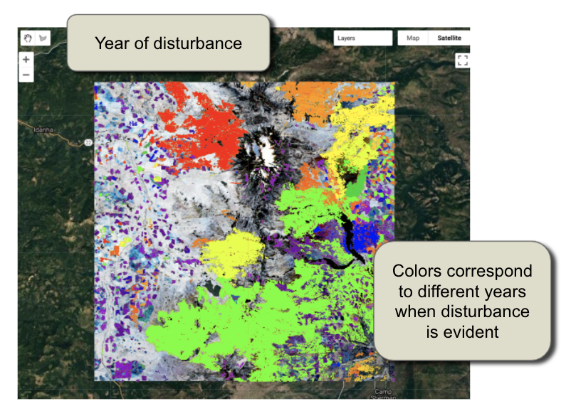
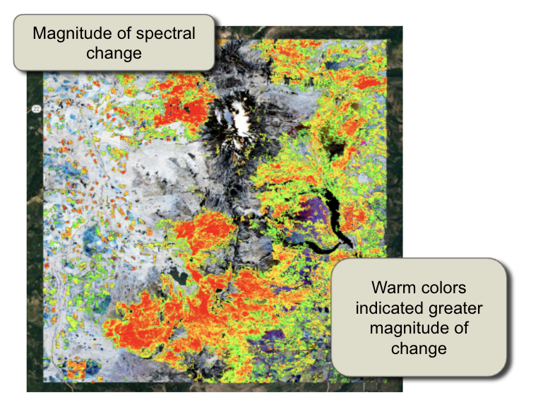
There are multiple layers of disturbance added to the map. Use the map layers checkboxes to change which is shown. Magnitude of disturbance, for example, is a map of the delta change between beginning and endpoints of the segments (Fig. 4.5.8).

Synthesis

In this chapter, you have learned how to work with annual time series to interpret regions of interest. Looking at annual snapshots of the landscape provides three key benefits: (1) the ability to view your area of interest without the clouds and noise that typically obscure single-day views; (2) gauge the amount by which the noise-dampened signal still varies from year to year in response to large-scale forcing mechanisms; and (3) the ability to view the response of landscapes as they recover, sometimes slowly, from disturbance.

To learn more about LandTrendr, see the assignments below.

Assignment 1. Find your own change processes of interest. First, navigate the map (zooming and dragging) to an area of the world where you are interested in a change process, and the spectral index that would capture it. Make sure the UI control panel is open to the Pixel Time-Series Options section. Next, click on the map in areas where you know change has occurred, and observe the spectral trajectories in the charts. Then, describe whether the change of interest is detectable in the spectral reflectance record, and what are its characteristics in different parts of the study area. .

Assignment 2: Find a pixel in your area of interest that shows a distinctive disturbance process, as you define it for your topic of interest. Adjust date ranges, parameters, etc. using the steps outlined in Section 1 above, and then answer these questions:

• Question 1. Which index and date range did you use?
• Question 2. Did you need to change fitting parameters to make the algorithm find the disturbance? If so, which ones, and why?
• Question 3. How do you know this is a disturbance?

Assignment 3. Switch the control panel in the GUI to Change Filter Options, and use the guidance in Section 2 to set parameters and make disturbance maps.  

• Question 4. Do the disturbance year and magnitude as mapped in the image match with what you would expect from the trajectory itself?
• Question 5. Can you change some of the filters to create a map where your disturbance process is not mapped? If so, what did you change?  
• Question 6. Can you change filters to create a map that includes a different disturbance process, perhaps subtler, longer duration, etc.? Find a pixel and use the “Pixel time series” plotter to look at the time series of those processes.

Assignment 4:  Return to the Pixel Time-Series Options section of the control panel, and navigate to a pixel in your area of interest that you believe would show a distinctive recovery or growth process, as you define it for your topic of interest. You may want to modify the index, parameters, etc. as covered in Section 1 to adequately capture the growth process with the fitted trajectories.

• Question 7. Did you use the same spectral index? If not, why?
• Question 8. Were the fitting parameters the same as those for disturbance? If not, what did you change, and why?
• Question 9. What evidence do you have that this is a vegetative growth signal?

Assignment 5. For vegetation gain mapping, switch the control panel back to Change Filter Options and use the guidance in Section 2 to set parameters, etc. to make maps of growth.

• Question 10. For the pixel or pixels you found for Assignment 3, does the year and magnitude as mapped in the “gain” image match with what you would expect from the trajectory itself?
• Question 11. Compare what the map looks like when you run it with and without the MMU filter. What differences do you see?
• Question 12. Try changing the recovery duration filter to a very high number (perhaps the full length of your archive) and to a very low number (say, one or two years). What differences do you see? 

CConclusion

This exercise provides a baseline sense of how the LandTrendr algorithm works. The key points are learning how to interpret change in spectral values in terms of the processes occurring on the ground, and then translating those into maps.

You can export the images you’ve made here using Download Options. Links to materials are available in the chapter checkpoints and LandTrendr documentation about both the GUI and the script-based versions of the algorithm. In particular, there are scripts that handle different components of the fitting and mapping process, and that allow you to keep track of the fitting and image selection criteria.

Feedback

To review this chapter and make suggestions or note any problems, please go now to bit.ly/EEFA-review. You can find summary statistics from past reviews at bit.ly/EEFA-reviews-stats.

References

Cloud-Based Remote Sensing with Google Earth Engine. (n.d.). CLOUD-BASED REMOTE SENSING WITH GOOGLE EARTH ENGINE. https://www.eefabook.org/

Cloud-Based Remote Sensing with Google Earth Engine. (2024). In Springer eBooks. https://doi.org/10.1007/978-3-031-26588-4

Kennedy RE, Yang Z, Cohen WB (2010) Detecting trends in forest disturbance and recovery using yearly Landsat time series: 1. LandTrendr - Temporal segmentation algorithms. Remote Sens Environ 114:2897–2910. https://doi.org/10.1016/j.rse.2010.07.008

Kennedy RE, Yang Z, Gorelick N, et al (2018) Implementation of the LandTrendr algorithm on Google Earth Engine. Remote Sens 10:691. https://doi.org/10.3390/rs10050691