Cloud-Based Remote Sensing with Google Earth Engine

Fundamentals and Applications

Part F6: Advanced Topics

Although you now know the most basic fundamentals of Earth Engine, there is still much more that can be done. The Part presents some advanced topics that can help expand your skill set for doing larger and more complex projects. These include tools for sharing code among users, scaling up with efficient project design, creating apps for non-expert users, and combining R with other information processing platforms.

Chapter F6.2: Scaling Up in Earth Engine

Authors

Jillian M. Deines, Stefania Di Tommaso, Nicholas Clinton, Noel Gorelick    

Overview

Commonly, when Earth Engine users move from tutorials to developing their own processing scripts, they encounter the dreaded error messages, “computation timed out” or “user memory limit exceeded.” Computational resources are never unlimited, and the team at Earth Engine has designed a robust system with built-in checks to ensure server capacity is available to everyone. This chapter will introduce general tips for creating efficient Earth Engine workflows that accomplish users’ ambitious research objectives within the constraints of the Earth Engine ecosystem. We use two example case studies: 1) extracting a daily climate time series for many locations across two decades, and 2) generating a regional, cloud-free median composite from Sentinel-2 imagery.

Learning Outcomes

• Understanding constraints on Earth Engine resource use.
• Becoming familiar with multiple strategies to scale Earth Engine operations.
• Managing large projects and multistage workflows.
• Recognizing when using the Python API may be advantageous to execute large batches of tasks.

Assumes you know how to:

• Import images and image collections, filter, and visualize (Part F1).
• Write a function and map it over an ImageCollection (Chap. F4.0).
• Export and import results as Earth Engine assets (Chap. F5.0).
• Understand distinctions among Image, ImageCollection, Feature and FeatureCollection Earth Engine objects (Part F1, Part F2, Part F5).
• Use the require function to load code from existing modules (Chap. F6.1).

Github Code link for all tutorials

This code base is collection of codes that are freely available from different authors for google earth engine.

Github Source

Introduction to Theory

Parts F1–F5 of this book have covered key remote sensing concepts and demonstrated how to implement them in Earth Engine. Most exercises have used local-scale examples to enhance understanding and complete tasks within a class-length time period. But Earth Engine’s power comes from its scalability—the ability to apply geospatial processing across large areas and many years.

How we go from small to large scales is influenced by Earth Engine’s design. Earth Engine runs on many individual computer servers, and its functions are designed to split up processing onto these servers. This chapter focuses on common approaches to implement large jobs within Earth Engine’s constraints. To do so, we first discuss Earth Engine’s underlying infrastructure to provide context for existing limits. We then cover four core concepts for scaling:

1. Using best coding practices.
2. Breaking up jobs across time.
3. Breaking up jobs across space.
4. Building a multipart workflow and exporting intermediate assets.

Earth Engine: Under the Hood

As you use Earth Engine, you may begin to have questions about how it works and how you can use that knowledge to optimize your workflow. In general, the inner workings are opaque to users. Typical fixes and approaches that data scientists use to manage memory constraints often don’t apply. It’s helpful to know what users can and cannot control, and how your scripts translate to Earth Engine’s server operations.

Earth Engine is a parallel, distributed system (see Gorelick et al. 2017), which means that when you submit tasks, it breaks up pieces of your query onto different processors to complete them more efficiently. It then collects the results and returns them to you. For many users, not having to manually design this parallel, distributed processing is a huge benefit. For some advanced users, it can be frustrating to not have better control. We’d argue that leaving the details up to Earth Engine is a huge time-saver for most cases, and learning to work within a few constraints is a good time investment.

One core concept useful to master is the relationship between client-side and server-side operations. Client-side operations are performed within your browser (for the JavaScript API Code Editor) or local system (for the Python API). These include things such as manipulating strings or numbers in JavaScript. Server-side operations are executed on Google’s servers and include all of the ee.* functions. By using the Earth Engine APIs—JavaScript or Python—you are building a chain of commands to send to the servers and later receive the result back. As much as possible, you want to structure your code to send all the heavy lifting to Google, and keep processing off of your local resources.

In other words, your work in the Code Editor is making a description of a computation. All ee objects are just placeholders for server-side objects—their actual value does not exist locally on your computer. To see or use the actual value, it has to be evaluated by the server. If you print an Earth Engine object, it calls getInfo to evaluate and return the value. In contrast, you can also work with JavaScript/Python lists or numbers locally, and do basic JavaScript/Python things to them, like add numbers together or loop over items. These are client-side objects. Whenever you bring a server-side object into your local environment, there’s a computational cost.

Table F6.2.1 describes some nuts and bolts about Earth Engine and their implications. Table F6.2.2 provides some of the existing limits on individual tasks.

Table F6.2.1 Characterics of Google Earth Engine and implications for running large jobs 

Table F6.2.2 Size limits for Earth Engine tasks

The Importance of Coding Best Practices

Good code scales better than bad code. But what is good code? Generally, for Earth Engine, good code means 1) using Earth Engine’s server-side operators; 2) avoiding multiple passes through the same image collection; 3) avoiding unnecessary conversions; and 4) setting the processing scale or sample numbers appropriate for your use case, i.e., avoid using very fine scales or large samples without reason.

We encourage readers to become familiar with the “Coding Best Practices” page in the online Earth Engine User Guide. This page provides examples for avoiding mixing client- and server-side functions, unnecessary conversions, costly algorithms, combining reducers, and other helpful tips. Similarly, the “Debugging Guide–Scaling Errors” page of the online Earth Engine User Guide covers some common problems and solutions.

In addition, some Earth Engine functions are more efficient than others. For example, Image.reduceRegions is more efficient than Image.sampleRegions, because sampleRegions regenerates the geometries under the hood. These types of best practices are trickier to enumerate and somewhat idiosyncratic. We encourage users to learn about and make use of the Profiler tab, which will track and display the resources used for each operation within your script. This can help identify areas to focus efficiency improvements. Note that the profiler itself increases resource use, so only use it when necessary to develop a script and remove it for production-level execution. Other ways to discover best practices include following/posting questions to GIS StackExchange or the Earth Engine Developer’s Discussion Group, swapping code with others, and experimentation.

Practicum

Section 1. Scaling Across Time

In this section we use an example of extracting climate data at features (points or polygons) to demonstrate how to scale an operation across many features (Sect. 1.1) and how to break up large jobs by time units when necessary (e.g, by years; Sect. 1.2).

1.1. Scaling Up with Earth Engine Operators: Annual Daily Climate Data

Earth Engine’s operators are designed to parallelize queries on the backend without user intervention. In many cases, they are sufficient to accomplish a scaling operation.

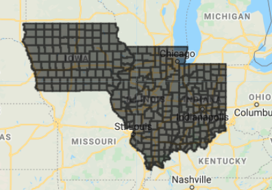
As an example, we will extract a daily time series of precipitation, maximum temperature, and minimum temperature for county polygons in the United States. We will use the GRIDMET Climate Reanalysis product (Abatzoglou 2013), which provides daily, 4000 m resolution gridded meteorological data from 1979 to the present across the contiguous United States. To save time for this practicum, we will focus on the states of Indiana, Illinois, and Iowa in the central United States, which together include 293 counties (Fig. F6.2.1).

This example uses the ee.Image.reduceRegions operator, which extracts statistics from an Image for each Feature (point or polygon) in a FeatureCollection. We will map the reduceRegions operator over each daily image in an ImageCollection, thus providing us with the daily climate information for each county of interest.

Note that although our example uses a climate ImageCollection, this approach transfers to any ImageCollection, including satellite imagery, as well as image collections that you have already processed, such as cloud masking (Chap. F4.3) or time series aggregation (Chap. F4.2).

First, define the FeatureCollection, ImageCollection, and time period:

Printing the size of the FeatureCollection indicates that there are 293 counties in our subset. Since we want to pull a daily time series for one year, our final dataset will have 106,945 rows—one for each county-day.

Note that from our county FeatureCollection, we select only the GEOID column, which represents a unique identifier for each record in this dataset. We do this here to simplify print outputs; we could also specify which properties to include in the export function (see below).

Next, load and filter the climate data. Note we adjust the end date to January 1 of the following year, rather than December 31 of the specified year, since the filterDate function has an inclusive start date argument and an exclusive end date argument; without this modification the output would lack data for December 31.

Now get the mean value for each climate attribute within each county feature. Here, we map the ee.Image.reduceRegions call over the ImageCollection, specifying an ee.Reducer.mean reducer. The reducer will apply to each band in the image, and it returns the FeatureCollection with new properties. We also add a 'date_ymd' time property extracted from the image to correctly associate daily values with their date. Finally, we flatten the output to reform a single FeatureCollection with one feature per county-day.

Note that we include a filter to remove feature-day rows that lacked data. While this is less common when using gridded climate products, missing data can be common when reducing satellite images. This is because satellite collections come in scene tiles, and each image tile likely does not overlap all of our features unless it has first been aggregated temporally. It can also occur if a cloud mask has been applied to an image prior to the reduction. By filtering out null values, we can reduce empty rows.

Now explore the result. If we simply print(sampledFeatures) we get our first error message: “User memory limit exceeded.” This is because we’ve created a FeatureCollection that exceeds the size limits set for interactive mode. How many are there? We could try print(sampledFeatures.size()), but due to the larger size, we receive a “Computation timed out” message—it’s unable to tell us. Of course, we know that we expect 293 counties x 365 days=106,945 features. We can, however, check that our reducer has worked as expected by asking Earth Engine for just one feature: print(sampledFeatures.limit(1)).

Here, we can see the precipitation, minimum temperature, and maximum temperature for the county with GEOID=17121 on January 1, 2020 (Fig. F6.2.2; note temperature is in Kelvin units).

Next, export the full FeatureCollection as a CSV to a folder in your Google Drive. Specify the names of properties to include. Build part of the filename dynamically based on arguments used for year and data scale, so we don’t need to manually modify the filenames.

Code Checkpoint F62a. The book’s repository contains a script that shows what your code should look like at this point.

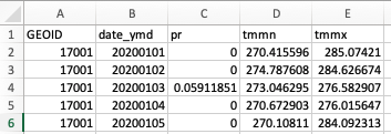
On our first export, this job took about eight minutes to complete, producing a dataset 6.8 MB in size. The data is ready for downstream use but may need formatting to suit the user’s goals. You can see what the exported CSV looks like in Fig. F6.2.3.

Using the Selectors Argument

There are two excellent reasons to use the selectors argument in your Export.table.toDrive call. First, if the argument is not specified, Earth Engine will generate the column names for the exported CSV from the first feature in your FeatureCollection. If that feature is missing properties, those properties will be dropped from the export for all features.

Perhaps even more important if you are seeking to scale up an analysis, including unnecessary columns can greatly increase file size and even processing time. For example, Earth Engine includes a .geo field that contains a GeoJSON description of each spatial feature. For non-simple geometries, the field can be quite large, as it lists coordinates for each polygon vertex. For many purposes, it’s not necessary to include this information for each daily record (here, 365 daily rows per feature).

For example, when we ran the same job as above but did not use the selectors argument, the output dataset was 5.7 GB (versus 6.8 MB!) and the runtime was slower. This is a cumbersomely large file, with no real benefit. We generally recommend dropping the .geo column and other unnecessary properties. To retain spatial information, a unique identifier for each feature can be used for downstream joins with the spatial data or other properties. If working with point data, latitude and longitude columns can be added prior to export to maintain easily accessible geographic information, although the .geo column for point data is far smaller than for irregularly shaped polygon features.

1.2. Scaling Across Time by Batching: Get 20 Years of Daily Climate Data

Above, we extracted one year of daily data for our 293 counties. Let’s say we want to do the same thing, but for 2001–2020. We have already written our script to flexibly specify years, so it’s fairly adaptable to this new use case:

If we only wanted a few years for a small number of features, we could just modify the startYear or endYear and proceed. Indeed, our current example is modest in size and number of features, and we were able to run 2001–2020 in one export job that took about two hours, with an output file size of 299 MB. However, with larger feature collections, or hourly data, we will again start to bump up against Earth Engine’s limits. Generally, jobs of this sort do not fail quickly—exports are allowed to run as long as they continue making progress (see Table F6.2.2). It’s not uncommon, however, for a large job to take well over 24 hours to run, or even to fail after more than 24 hours of run time, as it accumulates too many records or a single aggregation fails. For users, this can be frustrating.

We generally find it simpler to run several small jobs rather than one large job. Outputs can then be combined in external software. This avoids any frustration with long-running jobs or delayed failures, and it allows parts of the task to be run simultaneously. Earth Engine generally executes from 2–20 jobs per user at a time, depending on overall user load (although 20 is rare). As a counterpart, there is some overhead for generating separate jobs.

Important note: When running a batch of jobs, it may be tempting to use multiple accounts to execute subsets of your batch and thus get your shared results faster. However, doing so is a direct violation of the Earth Engine terms of service and can result in your account(s) being terminated.

For-Loops: They Are Sometimes OK

Batching jobs in time is a great way to break up a task into smaller units. Other options include batching jobs by spatial regions defined by polygons (see Sect. 2), or for computationally heavy tasks, batching by both space and time.

Because Export functions are client-side functions, however, you can’t create an export within an Earth Engine map command. Instead, we need to loop over the variable that will define our batches and create a set of export tasks.

But wait! Aren’t we supposed to avoid for-loops at all costs? Yes, within a computational chain. Here, we are using a loop to send multiple computational chains to the server.

First, we will start with the same script as in Sect. 1.1, but we will modify the start year. We will also modify the desired output filename to be a generic base filename, to which we will append the year for each task within the loop (in the next step).

Now modify the code in Sect. 1.1 to use a looping variable, i, to represent each year. Here, we are using standard JavaScript looping syntax, where i will take on each value between our startYear (2001) and our endYear (2020) for each loop through this section of code, thus creating 20 queries to send to Earth Engine’s servers.

Code Checkpoint F62b. The book’s repository contains a script that shows what your code should look like at this point.

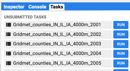
When we run this script, it builds our computational query for each year, creating a batch of 20 individual jobs that will show up in the Task pane (Fig. F6.2.4). Each task name includes the year, since we used our looping variable i to modify the base filename we specified.

We now encounter a downside to creating batch tasks within the JavaScript Code Editor: we need to click Run to execute each job in turn. Here, we made this easier by programmatically assigning each job the filename we want, so we can hold the Cmd/Ctrl key and click Run to avoid the export task option window and only need to click once per task. Still, one can imagine that at some number of tasks, one’s patience for clicking Run will be exceeded. We assume that number is different for everyone.

Note: If at any time you have submitted several tasks to the server but want to cancel them all, you can do so more easily from the Earth Engine Task Manager that is linked at the top of the Task pane. You can read about that task manager in the Earth Engine User Guide.

In order to auto-execute jobs in batch mode, we’d need to use the Python API. Interested users can see the Earth Engine User Guide Python API tutorial for further details about the Python API. 

Section 2. Scaling Across Space via Spatial Tiling

Breaking up jobs in space is another key strategy for scaling operations in Earth Engine. Here, we will focus on making a cloud-free composite from the Sentinel-2 Level 2A Surface Reflectance product. The approach is similar to that in Chap. F4.3, which explores cloud-free compositing. The main difference is that Landsat scenes come with a reliable quality band for each scene, whereas the process for Sentinel-2 is a bit more complicated and computationally intense (see below).

Our region of interest is the state of Washington in the United States for demonstration purposes, but the method will work at much larger continental scales as well.

Cloud Masking Approach

While we do not intend to cover the theory behind Sentinel-2 cloud masking, we do want to include a brief description of the process to convey the computational needs of this approach.

The Sentinel-2 Level 2A collection does not come with a robust cloud mask. Instead, we will build one from related products that have been developed for this purpose. Following the existing Sentinel-2 cloud masking tutorials in the Earth Engine guides, this approach requires three Sentinel-2 image collections:

• The Sentinel-2 Level 2A Surface Reflectance product. This is the dataset we want to use to build our final composite.
• The Sentinel-2 Cloud Probability Dataset, an ImageCollection that contains cloud probabilities for each Sentinel-2 scene.
• The Sentinel-2 Level 1C top-of-atmosphere product. This collection is needed to run the Cloud Displacement Index to identify cloud shadows, which is calculated using ee.Algorithms.Sentinel2.CDI (see Frantz et al. 2018 for algorithm description).

These three image collections all contain 10 m resolution data for every Sentinel-2 scene. We will join them based on their 'system:index' property so we can relate each Level 2A scene with the corresponding cloud probability and cloud displacement index. Furthermore, there are two ee.Image.projection steps to control the scale when calculating clouds and their shadows.

To sum up, the cloud masking approach is computationally costly, thus requiring some thought when applying it at scale.

2.1. Generate a Cloud-Free Satellite Composite: Limits to On-the-Fly Computing

Note: Our focus here is on code structure for implementing spatial tiling. Below, we import existing tested functions for cloud masking using the require command.

First, define our region and time of interest; then, load the module containing the cloud functions.

Next, load and filter our three Sentinel-2 image collections.

Now apply the cloud mask:

Next, generate and visualize the median composite:

Code Checkpoint F62c. The book’s repository contains a script that shows what your code should look like at this point.

After about 1–3 minutes, Earth Engine returns our composite to us on the fly (Fig. F6.2.5). Note that panning and zooming to a new area requires that Earth Engine must again issue the compositing request to calculate the image for new areas. Given the delay, this isn’t a very satisfying way to explore our composite.

Next, expand our view (set zoom to 9) to exceed the limits of on-the-fly computation (Fig. F6.2.6).

As you can see, this is an excellent candidate for an export task rather than running in “on-the-fly” interactive mode, as above.

2.2. Generate a Regional Composite Through Spatial Tiling

Our goal is to apply the cloud masking method in Sect. 2.1 to the state of Washington, United States. In our testing, we successfully exported one Sentinel-2 composite for this area in about nine hours, but for this tutorial, let’s presume we need to split the task up to be successful.

Essentially, we want to split our region of interest up into a regular grid. For each grid, we will export a composite image into a new ImageCollection asset. We can then load and mosaic our composite for use in downstream scripts (see below).

First, generate a spatial polygon grid (FeatureCollection) of desired size over your region of interest (see Fig. F6.2.7):

Next, create a new, empty ImageCollection asset to use as our export destination (Assets > New > Image Collection; Fig. F6.2.8). Name the image collection 'S2_composite_WA' and specify the asset location in your user folder (e.g., "path/to/your/asset/s2_composite_WA").

Specify the ImageCollection to export to, along with a base name for each image (the tile number will be appended in the batch export).

Extract grid numbers to use as looping variables. Note there is one getInfo call here, which should be used sparingly and never within a for-loop if you can help it. We use it to bring the number of grid cells we’ve generated onto the client-side to set up the for-loop over grids. Note that if your grid has too many elements, you may need a different strategy.

Batch generate a composite image task export for each grid via looping:

Code Checkpoint F62d. The book’s repository contains a script that shows what your code should look like at this point.

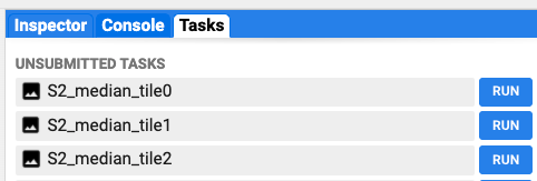
Similar to Sect. 1.2, we now have a list of tasks to execute. We can hold the Cmd/Ctrl key and click Run to execute each task (Fig. F6.2.9). Again, users with applications requiring large batches may want to explore the Earth Engine Python API, which is well-suited to batching work. The output ImageCollection is 35.3 GB, so you may not want to execute all (or any) of these tasks but can access our pre-generated image, as discussed below.

In addition to being necessary for very large regions, batch processing can speed things up for moderate scales. In our tests, tiles averaged about one hour to complete. Because three jobs in our queue were running simultaneously, we covered the full state of Washington in about four hours (compared to about nine hours when tested for the full state of Washington at once). Users should note, however, that there is also an overhead to spinning up each batch task. Finding the balance between task size and task number is a challenge for most Earth Engine users that becomes easier with experience.

In a new script, load the exported ImageCollection and mosaic for use.

Code Checkpoint F62e. The book’s repository contains a script that shows what your code should look like at this point.

Note the ease, speed, and joy of panning and zooming to explore the pre-computed composite asset (Fig. F6.2.10) compared to the on-the-fly version discussed in Sect. 2.1.

Section 3. Multistep Workflows and Intermediate Assets

Often, our goals require several processing steps that cannot be completed within one Earth Engine computational chain. In these cases, the best strategy becomes breaking down tasks into individual pieces that are created, stored in assets, and used across several scripts. Each sequential script creates an intermediate output, and this intermediate output becomes the input to the next script.

As an example, consider the land use classification task of identifying irrigated agricultural lands. This type of classification can benefit from several types of evidence, including satellite composites, aggregated weather information, soil information, and/or crop type locations. Individual steps for this type of work might include:

• Generating satellite composites of annual or monthly vegetation indices
• Processing climate data into monthly or seasonal values
• Generating random point locations from a ground truth layer for use as a feature training dataset and accuracy validation, and extracting composite and weather values at these features
• Training a classifier and applying it, possibly across multiple years; researchers will often implement multiple classifiers and compare the performance of different methods
• Implementing post-classification cleaning steps, such as removing “speckle”
• Evaluating accuracy at ground truth validation points, and against government statistics using total area per administrative boundary
• Exporting your work as spatial layers, visualizations, or other formats

Multipart workflows can become unwieldy to manage, particularly if there are multiple collaborators or the project has a long timeline; it can be difficult to remember why each script was developed and where it fits in the overall workflow.

Here, we provide tips for managing multipart workflows. These are somewhat opinionated and based largely on concepts from “Good Enough Practices in Scientific Computing” (Wilson et al. 2017). Ultimately, your personal workflow practices will be a combination of what works for you, what works for your larger team and organization, and, hopefully, what works for good documentation and reproducibility.

Tip 1. Create a repository for each project

The repository can be considered the fundamental project unit. In Earth Engine, sharing permissions are set for each individual repository, so this allows you to share a specific project with others (see Chap. F6.1).

By default, Earth Engine saves new scripts in a “default” repository specific for each user (users/<username>/default). You can create new repositories on the Scripts tab of the Code Editor (Fig. F6.2.11).

To adjust permissions for each repository, click on the Gear icon (Fig. F6.2.12):

For users familiar with version control, Earth Engine uses a git-based script manager, so each repository can also be managed, edited, and/or synced with your local copy or collaborative spaces like GitHub.

Tip 2. Make a separate script for each step, and make script file names informative and self-sorting

Descriptive, self-sorting filenames are an excellent “good enough” way to keep your projects organized. We recommend starting script names with zero-padded numeric values to take advantage of default ordering. Because we are generating assets in early scripts that are used in later scripts, it’s important to preserve the order of your workflow. The name should also include short descriptions of what the script does (Fig. F6.2.13).

Leaving some decimal places between successive scripts gives you the ability to easily insert any additional steps you didn’t originally anticipate. And zero-padding means your self-sorting still works once you move into double-digit numbers.

Other script organization strategies might involve including subfolders to collect scripts related to main steps. For example, one could have a subfolder “04_classifiers” to keep alternative classification scripts in one place, using a more tree-based file structure. Again, each user or group will develop a system that works for them. The important part is to have an organizational system.

Tip 3. Consider data types and file sizes when storing intermediates

Images and image collections are common intermediate file types, since generating satellite composites or creating land use classifications tends to be computationally intensive. These assets can also be quite large, depending on the resolution and region size. Recall that our single-year, subregional Sentinel-2 composite in Sect. 2 was about 23 GB.

Image values can be stored from 8-bit integers to 64-bit double floats (numbers with decimals). Higher bits allow for more precision, but have much larger file sizes and are not always necessary. For example, if we are generating a land use map with five classes, we can convert that to a signed or unsigned 8-bit integer using toInt8 or toUint8 prior to exporting to asset, which can accommodate 256 unique values. This results in a smaller file size. Selectively retaining only bands of interest is also helpful to reduce size.

For cases requiring decimals and precision, consider whether a 32-bit float will do the job instead of a 64-bit double—toFloat will convert an image to a 32-bit float. If you find you need to conserve storage, you can also scale float values and store as an integer image (image.multiply(100).toInt16(), for example). This would retain precision to the second decimal place and reduce file size by a factor of two. Note that this may require you to unscale the values in downstream use. Ultimately, the appropriate data type will be specific to your needs.

And of course, as mentioned above under “The Importance of Best Coding Practices,” be aware of the scale resolution you are working at, and avoid using unnecessarily high resolution when it’s not supported by either the input imagery or your research goals.

Tip 4. Consider Google Cloud Platform for hosting larger intermediates

If you are working with very large or very many files, you can link Earth Engine with Cloud Projects on Google Cloud Platform. See the Earth Engine documentation on “Setting Up Earth Engine Enabled Cloud Projects” for more information.

Synthesis

Earth Engine is built to be scaled. Scaling up working scripts, however, can present challenges when the computations take too long or return results that are too large or numerous. We have covered some key strategies to use when you encounter memory or computational limits. Generally, they involve 1) optimizing your code based on Earth Engine’s functions and infrastructure; 2) working at scales appropriate for your data, question, and region of interest, and not at higher resolutions than necessary; and 3) breaking up tasks into discrete units.

Feedback

To review this chapter and make suggestions or note any problems, please go now to bit.ly/EEFA-review. You can find summary statistics from past reviews at bit.ly/EEFA-reviews-stats.

References

Cloud-Based Remote Sensing with Google Earth Engine. (n.d.). CLOUD-BASED REMOTE SENSING WITH GOOGLE EARTH ENGINE. https://www.eefabook.org/

Cloud-Based Remote Sensing with Google Earth Engine. (2024). In Springer eBooks. https://doi.org/10.1007/978-3-031-26588-4

Abatzoglou JT (2013) Development of gridded surface meteorological data for ecological applications and modelling. Int J Climatol 33:121–131. https://doi.org/10.1002/joc.3413

Frantz D, Haß E, Uhl A, et al (2018) Improvement of the Fmask algorithm for Sentinel-2 images: Separating clouds from bright surfaces based on parallax effects. Remote Sens Environ 215:471–481. https://doi.org/10.1016/j.rse.2018.04.046

Gorelick N, Hancher M, Dixon M, et al (2017) Google Earth Engine: Planetary-scale geospatial analysis for everyone. Remote Sens Environ 202:18–27. https://doi.org/10.1016/j.rse.2017.06.031

Wilson G, Bryan J, Cranston K, et al (2017) Good enough practices in scientific computing. PLoS Comput Biol 13:e1005510. https://doi.org/10.1371/journal.pcbi.1005510