Human Applications

Built Environments

Cloud-Based Remote Sensing with Google Earth Engine

Fundamentals and Applications

Part A1: Human Applications

This Part covers some of the many Human Applications of Earth Engine. It includes demonstrations of how Earth Engine can be used in agricultural and urban settings, including for sensing the built environment and the effects it has on air composition and temperature. This Part also covers the complex topics of human health, illicit deforestation activity, and humanitarian actions.

Chapter A1.3: Built Environments

Author

Erin Trochim

Overview

The built environment consists of the human-made physical parts of the environment, including homes, buildings, streets, open spaces, and infrastructure. This chapter will focus on analyzing global infrastructure datasets.

Learning Outcomes

Quantifying road characteristics.
Comparing road and transmission line distributions.
Contrasting changes in impervious surfaces with flooding.
Understanding vector-based versus raster-based approaches.

Helps if you know how to:

Create a function for code reuse (Chap. F1.0).
Summarize an ImageCollection with reducers (Chap. F4.0, Chap. F4.1).
Filter a FeatureCollection to obtain a subset (Chap. F5.0, Chap. F5.1).
Convert between raster and vector data (Chap. F5.1).
Join elements of vector datasets together (Chap. F5.3).

Github Code link for all tutorials

This code base is collection of codes that are freely available from different authors for google earth engine.

Github Source

Introduction to Theory

Until the recent past, data about the built environment were mostly produced and managed at local and regional levels, and global datasets were very rare. Municipal, state, and national governments require easy access to data in order to plan, build, and maintain assets, which can be either privately or publicly owned. In the last decade, there has been a push to produce globally consistent data to support economic assessment and environmental transitions. The existence of this data makes it possible to explore the impact of factors including weather, climate, and growth over time.

Built environment datasets currently available in the Earth Engine Data Catalog include the Global Power Plant Database, Open Buildings V1 Polygons (which currently includes over half of Africa), and Global Artificial Impervious Area. Complementary environmental information includes the Global Flood Database. In addition, the Awesome GEE Community Datasets hosts the Global Roads Inventory Project, Global Power System, and Global Fixed Broadband and Mobile (Cellular) Network Performance collections.

As will be seen in the rest of this chapter, information on the built environment is most often stored as vector data: that is, as points, lines, and polygons. This format readily lends itself to representing, for example, bridges as points, roads as lines, and buildings as polygons. Many of the built environment datasets listed above now have both raster and vector components. It is useful to understand the utility of each of these formats and how to extract information between them and ancillary datasets.

Practicum

Section 1. Road Characteristics

We will start by calculating road length using the Global Roads Inventory Project (GRIP) dataset (Meijer et al. 2018). This dataset was created to provide a consistent global roadways dataset for environmental and biodiversity assessments. For this exercise, we will focus on examining the largest countries in Africa, North America, and Europe.

Start by importing the grip4 datasets into Earth Engine using the following code, and examine how they look in the Code Editor.

// Import roads data.
var grip4_africa=ee.FeatureCollection(
'projects/sat-io/open-datasets/GRIP4/Africa'),
grip4_north_america=ee.FeatureCollection(
'projects/sat-io/open-datasets/GRIP4/North-America'),
grip4_europe=ee.FeatureCollection(
'projects/sat-io/open-datasets/GRIP4/Europe');

// Check the roads data sizes.
print('Grip4 Africa size', grip4_africa.size());
print('Grip4 North America size', grip4_north_america.size());
print('Grip4 Europe size', grip4_europe.size());

// Display the roads data.
Map.addLayer(ee.FeatureCollection(grip4_africa).style({
color: '413B3A',
width: 1
}),{}, 'Grip4 Africa');
Map.addLayer(ee.FeatureCollection(grip4_north_america).style({
color: '413B3A',
width: 1
}),{}, 'Grip4 North America');
Map.addLayer(ee.FeatureCollection(grip4_europe).style({
color: '413B3A',
width: 1
}),{}, 'Grip4 Europe');

Using the Large Scale International Boundary dataset from the United States Office of the Geographer, below we will import the simplified country boundaries. After calculating the area enclosed by the boundary of each country, we will select Algeria, a quite large country with many roads.

// Import simplified countries.
var countries=ee.FeatureCollection('USDOS/LSIB_SIMPLE/2017');

// Add a function to calculate the feature's geometry area.
// Add the function as a property.
var addArea=function(feature){
return feature.set({
areaKm: feature.geometry().area().divide(1000 *
1000)
}); // km2 squared
};

// Map the area getting function over the FeatureCollection.
var countriesArea=countries.map(addArea);

// Filter to the largest country in Africa.
var Algeria=countriesArea.filter(ee.Filter.inList('country_na', [
'Algeria'
]));

// Display the selected countries.
Map.addLayer(Algeria.style({
fillColor: 'b5ffb4',
color: '00909F',
width: 1.0
}),{}, 'Algeria');

Next, we will calculate the road density for Algeria. For this example, we will implement a function to join the roads to each of the countries. The approach below joins the roads to the countries if there is spatial overlap between the features. Then, for each joined road in the specified country, an intersection is performed to keep only the portion of the road within the country. The length of the road is calculated and added as a property per feature, as is the road density per country.

// This function calculates the road length per country for the associated GRIP dataset.
var roadLength4Country=function(country, grip4){

// Join roads to countries.
var intersectsFilter=ee.Filter.intersects({
leftField: '.geo',
rightField: '.geo',
maxError: 10
});

var grip4Selected=grip4.filterBounds(country);

var countriesWithRds=ee.Join.saveAll('roads').apply({
primary: country,
secondary: grip4Selected,
condition: intersectsFilter
}).filter(ee.Filter.neq('roads', null));

// Return country with calculation of roadLength and roadsPerArea.
return countriesWithRds.map(function(country){
var roadsList=ee.List(country.get('roads'));
var roadLengths=roadsList.map(function(road){
return ee.Feature(road).intersection(
country, 10).length(10);
});
var roadLength=ee.Number(roadLengths.reduce(ee
.Reducer.sum()));
return country.set({
roadLength: roadLength.divide(
1000), // Convert to km.
roadsPerArea: roadLength.divide(ee
.Number(country.get('areaKm'))
)
});
}).select(['country_na', 'areaKm', 'roadLength',
'roadsPerArea'
]);
};

// Apply the road length function to Algeria.
var roadLengthAlgeria=roadLength4Country(Algeria, grip4_africa);

Print the roads per area in Algeria.

// Print the road statistics for Algeria.
print('Roads statistics in Algeria', roadLengthAlgeria);

Question 1. How many roads are there in Africa? Hint: Check the size of the grip4 Africa dataset.

Question 2. Which continent has the most roads: Africa, Europe, or North America?

Question 3. How many roads per square kilometer are there in Algeria?

Question 4. What is the total road length in kilometers in Algeria?

Code Checkpoint A13a. The book’s repository contains a script that shows what your code should look like at this point.

Earth Engine is powerful, but its processing power is not infinite. If you try applying the same code to countries such as Canada and France, it doesn’t run very well interactively due to the enormous size of the request. To successfully execute long-running, complex tasks, you can export results. Exporting forces Earth Engine to continue to run for a very long time; in that case, you can’t see the results interactively, but you will be able to get an answer for even very large problems, and then load the exported data. An example of this is shown below.

// Export feature collection to drive.
Export.table.toDrive({
collection: roadLengthAlgeria,
description: 'RoadStatisticsforAlgeria',
selectors: ['country_na', 'roadLength', 'roadsPerArea']
});

Let’s think about how to simplify this analysis, to see if we can optimize the computation in an interactive environment. Print the first feature of the grip4 Africa feature collection and display it using the following commands.

// Print the first feature of the grip4 Africa feature collection.
print(grip4_africa.limit(1));

Map.setCenter(-0.759, 9.235, 6);
Map.addLayer(grip4_africa.limit(1),
{},
'Road length comparison');

You can find the road in northern Ghana as shown in Fig. A1.3.1.

Fig. A1.3.1 Exploring the GRIP datasets by visualizing the first feature in the Africa region. According to the feature properties, the road is 0.76, but the unit is not specified. Compare this to the scale at the bottom of the Map panel in the Code Editor.

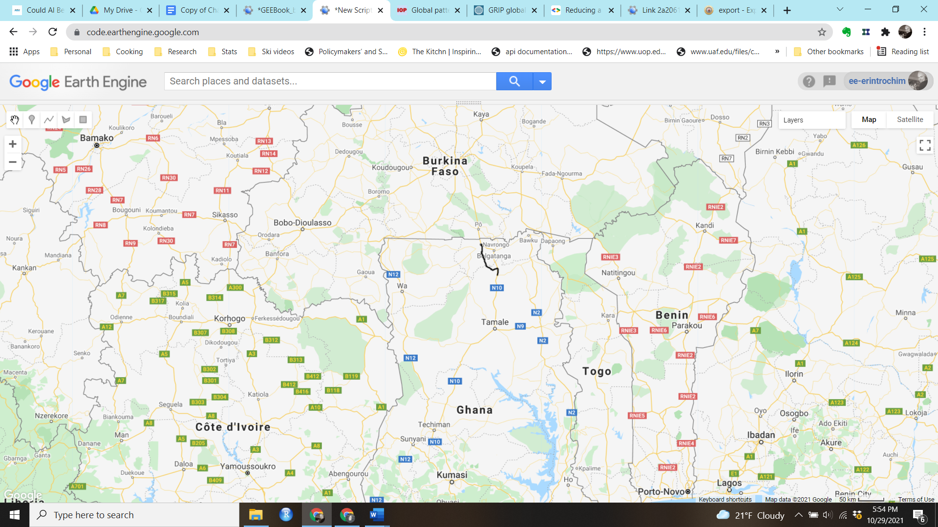
In the Console, examine the properties of the road. Notice there is an existing column called Shape_Leng. The length of each road appears to have already been precalculated and included as a value. The length of this road is given as 0.76, but the unit is not specified. This looks suspicious in comparison to the scale—the road is obviously longer than 0.76 meters, kilometers, or miles. It is easy to recalculate the length of the lines: use the following code to do so and compare the results.

// This function adds line length in km.
var addLength=function(feature){
return feature.set({
lengthKm: feature.length().divide(1000)
});
};

// Calculate the line lengths for all roads in Africa.
var grip4_africaLength=grip4_africa.map(addLength);

// Compare with other values.
print('Calculated road length property', grip4_africaLength.limit(1));

The road in Ghana has a new calculated length of about 84 km, which looks accurate.

Repeat the road calculation analysis, but examine each step. First, filter the road data in Africa for Algeria. Visualize the result, taking note of whether any roads are included that originate in Algeria but extend into other countries. Then, reduce the lengthKm column and calculate the sum in the filtered Algeria road data.

// Repeat the analysis to calculate the length of all roads.
// Filter the table geographically: only keep roads in Algeria.
var grip4_Algeria=grip4_africaLength.filterBounds(Algeria);

// Visualize the output.
Map.addLayer(grip4_Algeria.style({
color: 'green',
width: 2.0
}),{}, 'Algeria roads');

// Sum the lengths for roads in Algeria.
var sumLengthKmAlgeria=ee.Number(
// Reduce to get the sum.
grip4_Algeria.reduceColumns(ee.Reducer.sum(), ['lengthKm'])
.get('sum')
);

// Print the result.
print('Length of all roads in Algeria', sumLengthKmAlgeria);

Question 5. What is the total recalculated road length in kilometers in Algeria?

Question 6. Is this higher or lower than the first value?

Code Checkpoint A13b. The book’s repository contains a script that shows what your code should look like at this point.

The difference in values when recalculating is due to extra roads being included in the second calculation. This was due to skipping the joining and intersection of the Algeria feature collection. Using only filterBounds to approximate the road limits was not as accurate.

Let’s try another method to make this more computationally efficient. Rasterize the roads by interpolating the current feature collection into an image, and use reduceRegions to calculate the area of the road pixels. For this exercise, set the scale as 100 m. In order to convert the area into the appropriate dimension and units, divide the results by 1000 and apply a square root to transform the length into kilometers.

// Repeat the analysis again to calculate length of all roads using rasters.
// Convert to raster.
var empty=ee.Image().float();

var grip4_africaRaster=empty.paint({
featureCollection: grip4_africaLength,
color: 'lengthKm'
}).gt(0);

Map.addLayer(grip4_africaRaster,{
palette: ['orange'],
max: 1
}, 'Rasterized roads');

// Add reducer output to the features in the collection.
var AlgeriaRoadLength=ee.Image.pixelArea()
.addBands(grip4_africaRaster)
.reduceRegions({
collection: Algeria,
reducer: ee.Reducer.sum(),
scale: 100,
}).map(function(feature){
var num=ee.Number.parse(feature.get('area'));
return feature.set('length', num.divide(1000).sqrt()
.round());
});

// Print the first feature to illustrate the result.
print('Length of all roads in Algeria calculated via rasters', ee
.Number(AlgeriaRoadLength.first().get('length')));

Notice this value is about 13%, or 7000 km, lower than the first estimate.

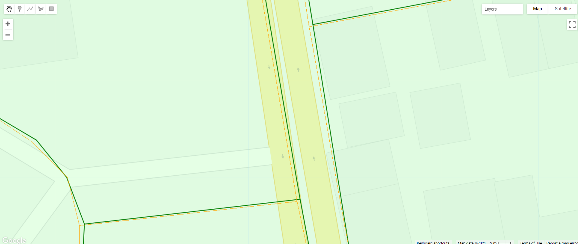
Take a look at the rasterized roads visualization. With no scale set, it looks very similar to the vectors. Zoom in to an area like the example in Fig. A1.3.2 and examine the structure of the vectors, rasters, and roads themselves. Note that, in some areas, divided roads are represented by two separate features (vectors). The initial rasters match the scale of the vector. One 100 m pixel, though, would cover both roads and represent only a single unit length. Understanding how the data represents the actual built environment is critical for accuracy and precision estimates. There is also a tradeoff in computation time and whether the calculations can be performed on the fly.

Fig. A1.3.2 Examining roads from the GRIP dataset as features (in green) versus rasters (in orange) overlaid with transparency on the Map view. There can be offset between datasets and different spatial shapes (lines, polygons, and rasters).

The advantage to this approach is that the analysis can be performed interactively across much larger areas. We will test this by calculating total road length for the largest countries in Africa, North America, and Europe, which are Algeria, Canada, and France.

// Calculate line lengths for all roads in North America and Europe.
var grip4_north_americaLength=grip4_north_america.map(addLength);
var grip4_europeLength=grip4_europe.map(addLength);

// Merge all vectors.
var roadLengthMerge=grip4_africaLength.merge(
grip4_north_americaLength).merge(grip4_europeLength);

// Convert to raster.
var empty=ee.Image().float();

var roadLengthMergeRaster=empty.paint({
featureCollection: roadLengthMerge,
color: 'roadsPerArea'
}).gt(0);

// Filter to largest countries in Africa, North America and Europe.
var countriesSelected=countries.filter(ee.Filter.inList(
'country_na', ['Algeria', 'Canada', 'France']));

// Clip image to only countries of analysis.
var roadLengthMergeRasterClipped=roadLengthMergeRaster
.clipToCollection(countriesSelected);

// Add reducer output to the features in the collection.
var countriesRoadLength=ee.Image.pixelArea()
.addBands(roadLengthMergeRasterClipped)
.reduceRegions({
collection: countriesSelected,
reducer: ee.Reducer.sum(),
scale: 100,
}).map(function(feature){
var num=ee.Number.parse(feature.get('area'));
return feature.set('length', num.divide(1000).sqrt()
.round());
});

// Compute totaled road lengths in km, grouped by country.
print('Length of all roads in Canada', countriesRoadLength.filter(ee
.Filter.equals('country_na', 'Canada')).aggregate_sum(
'length'));
print('Length of all roads in France', countriesRoadLength.filter(ee
.Filter.equals('country_na', 'France')).aggregate_sum(
'length'));

Question 7. Which country has the highest total length of roads?

Question 8. Explore the effect of the scale value by reprojecting the rasterized roads (for example, Map.addLayer(grip4_africaRaster.reproject({crs: 'EPSG:4326', scale: 100}),{palette: ['orange'], max: 1}, 'Rasterized roads 100 m')). Does increasing the scale result in an over- or underestimation of roads? What is an optimal scale to still allow the large calculations to run in real time?

Code Checkpoint A13c. The book’s repository contains a script that shows what your code should look like at this point.

Section 2. Road and Transmission Line Comparison

Next, let’s compare the overlap between roads and transmission lines, which often are found in the same vicinity. We will test this concept by examining the Global Power System data (Arderne et al. 2020).

Let’s start by creating a new script and importing data into the Code Editor. As in the first exercise, import the GRIP road datasets. We will reuse the same addLength function from the previous exercise and apply it to roads in Africa. Then, convert the roads to a raster using length in kilometers as the pixel value.

// Import roads data.
var grip4_africa=ee.FeatureCollection(
'projects/sat-io/open-datasets/GRIP4/Africa'),
grip4_europe=ee.FeatureCollection(
'projects/sat-io/open-datasets/GRIP4/Europe'),
grip4_north_america=ee.FeatureCollection(
'projects/sat-io/open-datasets/GRIP4/North-America');

// Add a function to add line length in km.
var addLength=function(feature){
return feature.set({
lengthKm: feature.length().divide(1000)
}); // km;
};

// Calculate line lengths for all roads in Africa.
var grip4_africaLength=grip4_africa.map(addLength);

// Convert the roads to raster.
var empty=ee.Image().float();

var grip4_africaRaster=empty.paint({
featureCollection: grip4_africaLength,
color: 'lengthKm'
});

Next, import the simplified countries again and filter the feature collection, this time to all countries on the continent of Africa.

Import the global power system data that represents transmission lines. For this exercise, we will use both the OpenStreetMap and predicted values in this dataset. Validation of this dataset included several parts of Africa, so it tends to have higher accuracy here than in other parts of the world like the Arctic.

Apply a filter to the transmission lines data to limit the analysis to Africa. Calculate the length of the lines and convert it to rasters, as with the roads data.

// Import simplified countries.
var countries=ee.FeatureCollection('USDOS/LSIB_SIMPLE/2017');

// Filter to Africa.
var Africa=countries.filter(ee.Filter.eq('wld_rgn', 'Africa'));

// Import global power transmission lines.
var transmission=ee.FeatureCollection(
'projects/sat-io/open-datasets/predictive-global-power-system/distribution-transmission-lines'
);

// Filter transmission lines to Africa.
var transmissionAfrica=transmission.filterBounds(Africa);

// Calculate line lengths for all transmission lines in Africa.
var transmissionAfricaLength=transmissionAfrica.map(addLength);

// Convert the transmission lines to raster.
var transmissionAfricaRaster=empty.paint({
featureCollection: transmissionAfricaLength,
color: 'lengthKm'
});

Question 9. In this exercise, we are rasterizing our feature collections to calculate spatial association indicators. If the data were left as a feature collection, what would be the simplest way of comparing the two datasets in a similar way?

Code Checkpoint A13d. The book’s repository contains a script that shows what your code should look like at this point.

In order to compare the road and transmission line rasters, they need to be stacked together into a single image. It is a good idea to rename the bands to keep track of the input values. Clip this dataset to the Africa feature collection in order to minimize computation in the following steps.

// Add roads and transmission lines together into one image.
// Clip to Africa feature collection.
var stack=grip4_africaRaster
.addBands(transmissionAfricaRaster)
.rename(['roads', 'transmission'])
.clipToCollection(Africa);

Next, use the following code to calculate the spatial statistics’ local Geary’s C (Anselin 2010). This will indicate clustering due to spatial autocorrelation. In this case, we are comparing whether roads and transmission lines are located together. Geary’s C values of −1 indicate dispersion, while those of 1 indicate clustering.

// Calculate spatial statistics: local Geary's C.
// Create a list of weights for a 9x9 kernel.
var list=[1, 1, 1, 1, 1, 1, 1, 1, 1];

// The center of the kernel is zero.
var centerList=[1, 1, 1, 1, 0, 1, 1, 1, 1];

// Assemble a list of lists: the 9x9 kernel weights as a 2-D matrix.
var lists=[list, list, list, list, centerList, list, list, list,
list
];

// Create the kernel from the weights.
// Non-zero weights represent the spatial neighborhood.
var kernel=ee.Kernel.fixed(9, 9, lists, -4, -4, false);

// Use the max among bands as the input.
var maxBands=stack.reduce(ee.Reducer.max());

// Convert the neighborhood into multiple bands.
var neighs=maxBands.neighborhoodToBands(kernel);

// Compute local Geary's C, a measure of spatial association
// - 0 indicates perfect positive autocorrelation/clustered
// - 1 indicates no autocorrelation/random
// - 2 indicates perfect negative autocorrelation/dispersed
var gearys=maxBands.subtract(neighs).pow(2).reduce(ee.Reducer.sum())
.divide(Math.pow(9, 2));

// Convert to a -/+1 scale by: calculating C*=1 - C
// - 1 indicates perfect positive autocorrelation/clustered
// - 0 indicates no autocorrelation/random
// - -1 indicates perfect negative autocorrelation/dispersed
var gearysStar=ee.Image(1).subtract(gearys);

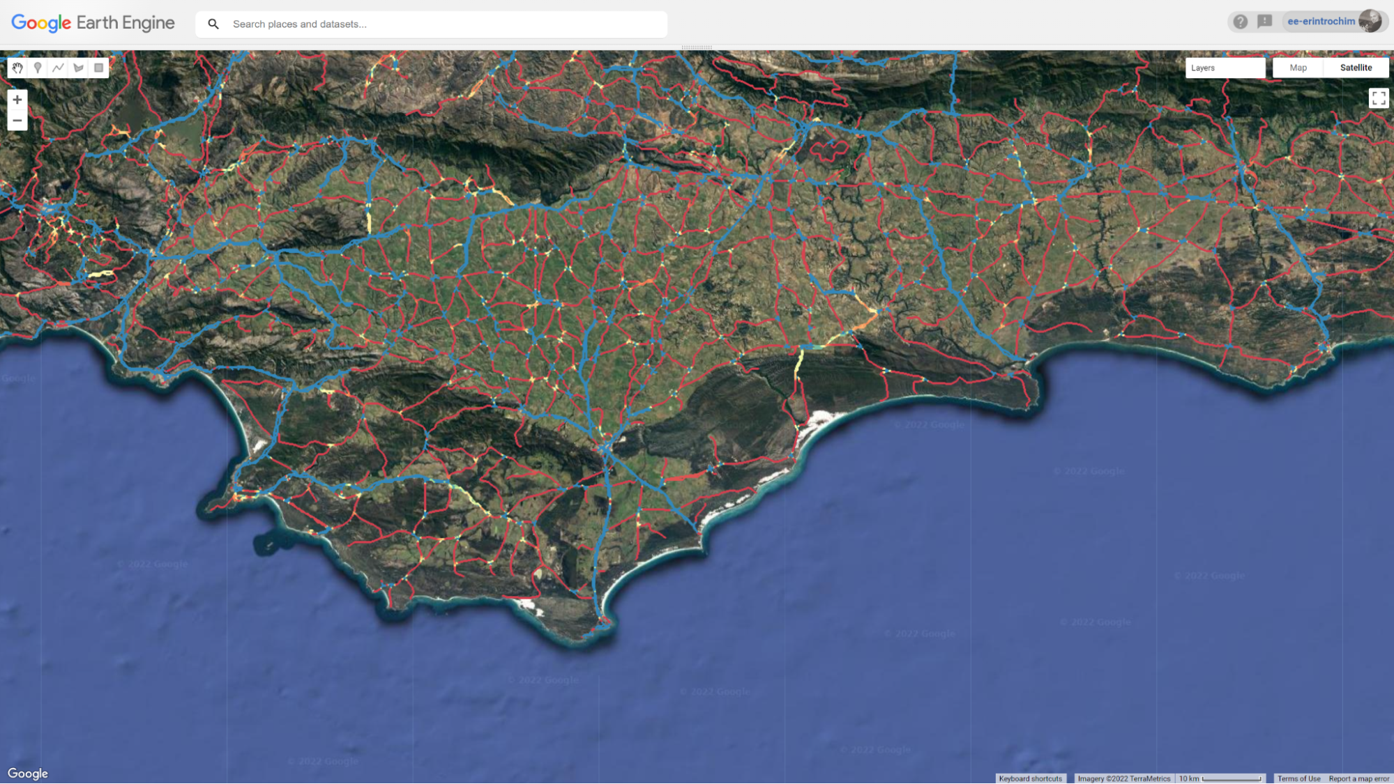
Examine the output by creating a custom palette and using a high-contrast basemap. The example illustrated in Fig. A1.3.3 shows how to add a focal max to the final image in order to better visualize the results as a raster. The color blue indicates values toward −1 and therefore dispersion, while red represents values toward 1 and therefore spatially clustered.

// Import palettes.
var palettes=require('users/gena/packages:palettes');

// Create custom palette, blue is negative while red is positive autocorrelation/clustered.
var palette=palettes.colorbrewer.Spectral[7].reverse();

// Normalize the image and add it to the map.
var visParams={
min: -1,
max: 1,
palette: palette
};

// Display the image.
Map.setCenter(19.8638, -34.5705, 10);
Map.addLayer(gearysStar.focalMax(1), visParams, 'local Gearys C*');

Fig. A1.3.3 Results of Geary’s C* spatial autocorrelation between roads and transmission lines in South Africa. Red indicates clustering, while blue indicates dispersion. Shorter stretches in this example appear to have more co-located linear infrastructure.

Question 10. What are the characteristics of the roads and transmission lines that are clustered?

Question 11. In this exercise, we are rasterizing our feature collections to calculate local indicators of spatial association. If the data were left as a feature collection, what would be the simplest way of comparing the two datasets?

Code Checkpoint A13e. The book’s repository contains a script that shows what your code should look like at this point.

Save your script for your own future use, as outlined in Chap. F1.0. Then, refresh the Code Editor to begin with a new script for the next section.

Section 3. Impervious Surfaces and Flooding

For our final exercise, we will compare impervious surfaces and flooding over time in a new script. The Global Artificial Impervious Area dataset captures annual change information at a 30 m resolution of impervious surface area from 1985 to 2018 (Gong et al. 2020). Impervious surfaces can include a variety of built environment surfaces, including anything with pavement or water-resistant materials—roads, sidewalks, airports, parking lots, ports, distribution centers, rooftops, etc. Artificial impervious areas are important because they are a clear representation of human settlements (Gong et al. 2020).

We will compare these impervious areas with the Global Flood Database, which describes flood extent and population characteristics for 913 large flood events from 2000 to 2018 at 250 m resolution (Tellman et al. 2021).

In this example, let’s compare the area of impervious surfaces in 2000 versus 2018 over the satellite-observed historical floodplain. Below, we will load the Global Artificial Impervious Area dataset, to display the images and compare the data for the two dates.

// Import Tsinghua FROM-GLC Year of Change to Impervious Surface
var impervious=ee.Image('Tsinghua/FROM-GLC/GAIA/v10');

// Use the change year values found in the band.
// The change year values is described here:
// https://developers.google.com/earth-engine/datasets/catalog/Tsinghua_FROM-GLC_GAIA_v10#bands
// Select only those areas which were impervious by 2000.
var impervious2000=impervious.gte(19);

// Select only those areas which were impervious by 2018.
var impervious2018=impervious.gte(1);

Map.setCenter(-98.688, 39.134, 5);

// Display the images.
Map.addLayer(
impervious2000.selfMask(),
{
min: 0,
max: 1,
palette: ['014352', '856F96']
},
'Impervious Surface 2000');

Map.addLayer(
impervious2018.selfMask(),
{
min: 0,
max: 1,
palette: ['014352', '1A492C']
},
'Impervious Surface 2018');

Subtract the two images to find the change between 2018 and 2000, and again display the results:

// Calculate the difference between impervious areas in 2000 and 2018.
var imperviousDiff=impervious2018.subtract(impervious2000);

Map.addLayer(
imperviousDiff.selfMask(),
{
min: 0,
max: 1,
palette: ['014352', 'FFBF00']
},
'Impervious Surface Diff 2000-18');

Import the Global Flood Database. Select the 'flooded' band and sum all values to create the satellite-observed historical floodplain. Mask out the areas of permanent water in the floodplain using the JRC Global Surface Water dataset included in the Global Flood Database as the 'jrc_perm_water' band. The JRC data uses the dataset’s original 'transition' band. Display the final floodplain results:

// Import the Global Flood Database v1 (2000-2018).
var gfd=ee.ImageCollection('GLOBAL_FLOOD_DB/MODIS_EVENTS/V1');

// Map all floods to generate the satellite-observed historical flood plain.
var gfdFloodedSum=gfd.select('flooded').sum();

// Mask out areas of permanent water.
var gfdFloodedSumNoWater=gfdFloodedSum.updateMask(gfd.select(
'jrc_perm_water').sum().lt(1));

var durationPalette=['C3EFFE', '1341E8', '051CB0', '001133'];

Map.addLayer(
gfdFloodedSumNoWater.selfMask(),
{
min: 0,
max: 10,
palette: durationPalette
},
'GFD Satellite Observed Flood Plain');

Now we’ll calculate which states have been developing the greatest amounts of impervious surfaces in floodplain areas. Start by masking out areas in the imperviousDiff image that are not in the floodplains (gfdFloodedSumNoWater greater than or equal to 1). Then, we will import the first-order administrative Global Administrative Unit Layers from the UN Food and Agriculture Organization. Filter this feature collection to administrative names ('ADM0_NAME') equal to 'United States of America'. Create an area image by multiplying the impervious difference flood image by pixel area. Apply a reduceRegions reducer to the area image using the United States feature collection and an initial scale of 100 m. Sort the output sum by descending order and get only the five highest states. Print the output.

// Mask areas in the impervious difference image that are not in flood plains.
var imperviousDiffFloods=imperviousDiff
.updateMask(gfdFloodedSumNoWater.gte(1));

// Which state has built the most area in the flood plains?
// Import FAO countries with first level administrative units.
var countries=ee.FeatureCollection('FAO/GAUL/2015/level1');

// Filter to the United States.
var unitedStates=countries.filter(ee.Filter.eq('ADM0_NAME',
'United States of America'));

// Calculate the image area.
var areaImage=imperviousDiffFloods.multiply(ee.Image.pixelArea());

// Sum the area image for each state.
var unitedStatesImperviousDiffFlood=areaImage.reduceRegions({
collection: unitedStates,
reducer: ee.Reducer.sum(),
scale: 100,
}) // Sort descending.
.sort('sum', false)
// Get only the 5 highest states.
.limit(5);

// Print state statistics for change in impervious area in flood plain.
print('Impervious-flood change statistics for states in US',
unitedStatesImperviousDiffFlood);

Question 12. Which state built the highest amount of impervious surfaces on satellite-derived floodplains between 2000 and 2018?

Question 13. Which state built the lowest amount of impervious surfaces on satellite-derived floodplains between 2000 and 2018?

Code Checkpoint A13f. The book’s repository contains a script that shows what your code should look like at this point.

Synthesis

Assignment 1. Rerun the first exercise using the first-order administrative Global Administrative Unit Layers. Try selecting different countries to explore which ones have the highest road density. You will likely need to save the output in order to run this analysis.

Assignment 2. Compute local Geary’s C for roads and transmission lines on other continents. Which continent appears to have the strongest clustering?

Assignment 3. Examine the Global Flood Database in relation to roads in an area of your choice. Try country-level analysis. Which country in your area has the highest proportion of roads potentially affected by flooding?

Conclusion

In this chapter, we have examined data from the built environment. We started by looking at characteristics of roads, then examined the interactions between roads and transmission lines, and finished by examining where built environments were most commonly developed in floodplains. Data in the built environment can be found in both vector and raster forms. We examined analysis using both forms, including rasterizing vector data. Our analysis also focused on larger-scale spatial analysis at the state, country, and continental level. Understanding how to do this type of analysis allows us to develop a better understanding of these systems as more seamless data across temporal and spatial dimensions continues to become available.

Feedback

To review this chapter and make suggestions or note any problems, please go now to bit.ly/EEFA-review. You can find summary statistics from past reviews at bit.ly/EEFA-reviews-stats.

References

Cloud-Based Remote Sensing with Google Earth Engine. (n.d.). CLOUD-BASED REMOTE SENSING WITH GOOGLE EARTH ENGINE. https://www.eefabook.org/

Cloud-Based Remote Sensing with Google Earth Engine. (2024). In Springer eBooks. https://doi.org/10.1007/978-3-031-26588-4

Anselin L (1995) Local indicators of spatial association—LISA. Geogr Anal 27:93–115. https://doi.org/10.1111/j.1538-4632.1995.tb00338.x

Arderne C, Zorn C, Nicolas C, Koks EE (2020) Predictive mapping of the global power system using open data. Sci Data 7:1–12. https://doi.org/10.1038/s41597-019-0347-4

Gong P, Li X, Wang J, et al (2020) Annual maps of global artificial impervious area (GAIA) between 1985 and 2018. Remote Sens Environ 236:111510. https://doi.org/10.1016/j.rse.2019.111510

Meijer JR, Huijbregts MAJ, Schotten KCGJ, Schipper AM (2018) Global patterns of current and future road infrastructure. Environ Res Lett 13:64006. https://doi.org/10.1088/1748-9326/aabd42

Tellman B, Sullivan JA, Kuhn C, et al (2021) Satellite imaging reveals increased proportion of population exposed to floods. Nature 596:80–86. https://doi.org/10.1038/s41586-021-03695-w