Cloud-Based Remote Sensing with Google Earth Engine
Fundamentals and Applications

Part F4: Interpreting Image Series
One of the paradigm-changing features of Earth Engine is the ability to access decades of imagery without the previous limitation of needing to download all the data to a local disk for processing. Because remote-sensing data files can be enormous, this used to limit many projects to viewing two or three images from different periods. With Earth Engine, users can access tens or hundreds of thousands of images to understand the status of places across decades.
Chapter F4.3: Clouds and Image Compositing
Authors:
Txomin Hermosilla, Saverio Francini, Andréa P. Nicolau, Michael A. Wulder, Joanne C. White, Nicholas C. Coops, Gherardo Chirici
Overview
The purpose of this chapter is to provide necessary context and demonstrate different approaches for image composite generation when using data quality flags, using an initial example of removing cloud cover. We will examine different filtering options, demonstrate an approach for cloud masking, and provide additional opportunities for image composite development. Pixel selection for composite development can exclude unwanted pixels—such as those impacted by cloud, shadow, and smoke or haze—and can also preferentially select pixels based upon proximity to a target date or a preferred sensor type.
Learning Outcomes
- Understanding and applying satellite-specific cloud mask functions.
- Incorporating images from different sensors.
- Using focal functions to fill in data gaps.
Assumes you know how to:
- Import images and image collections, filter, and visualize (Part F1).
- Perform basic image analysis: select bands, compute indices, create masks (Part F2).
- Use band scaling factors (Chap. F3.1).
- Perform pixel-based transformations (Chap. F3.1).
- Use neighborhood-based image transformations (Chap. F3.2).
- Write a function and map it over an ImageCollection (Chap. F4.0).
- Summarize an ImageCollection with reducers (Chap. F4.0, Chap. F4.1).
Github Code link for all tutorials
This code base is collection of codes that are freely available from different authors for google earth engine.
Introduction to Theory
In many respects, satellite remote sensing is an ideal source of data for monitoring large or remote regions. However, cloud cover is one of the most common limitations of optical sensors in providing continuous time series of data for surface mapping and monitoring. This is particularly relevant in tropical, polar, mountainous, and high-latitude areas, where clouds are often present. Many studies have addressed the extent to which cloudiness can restrict the monitoring of various regions (Zhu and Woodcock 2012, 2014; Eberhardt et al. 2016; Martins et al. 2018).
Clouds and cloud shadows reduce the view of optical sensors and completely block or obscure the spectral response from Earth’s surface (Cao et al. 2020). Working with pixels that are cloud-contaminated can significantly influence the accuracy and information content of products derived from a variety of remote sensing activities, including land cover classification, vegetation modeling, and especially change detection, where unscreened clouds might be mapped as false changes (Braaten et al. 2015, Zhu et al. 2015). Thus, the information provided by cloud detection algorithms is critical to exclude clouds and cloud shadows from subsequent processing steps.
Historically, cloud detection algorithms derived the cloud information by considering a single date-image and sun illumination geometry (Irish et al. 2006, Huang et al. 2010). In contrast, current, more accurate cloud detection algorithms are based on the analysis of Landsat time series (Zhu and Woodcock 2014, Zhu and Helmer 2018). Cloud detection algorithms inform on the presence of clouds, cloud shadows, and other atmospheric conditions (e.g., presence of snow). The presence and extent of cloud contamination within a pixel is currently provided with Landsat and Sentinel-2 imagery as ancillary data via quality flags at the pixel level. Additionally, quality flags also inform on other acquisition-related conditions, including radiometric saturation and terrain occlusion, which enables us to assess the usefulness and convenience of inclusion of each pixel in subsequent analyses. The quality flags are ideally suited to reduce users’ manual supervision and maximize the automatic processing approaches.
Most automated algorithms (for classification or change detection, for example) work best on images free of clouds and cloud shadows, that cover the full area without spatial or spectral inconsistencies. Thus, the image representation over the study area should be seamless, containing as few data gaps as possible. Image compositing techniques are primarily used to reduce the impact of clouds and cloud shadows, as well as aerosol contamination, view angle effects, and data volumes (White et al. 2014). Compositing approaches typically rely on the outputs of cloud detection algorithms and quality flags to include or exclude pixels from the resulting composite products (Roy et al. 2010). Epochal image composites help overcome the limited availability of cloud-free imagery in some areas, and are constructed by considering the pixels from all images acquired in a given period (e.g., season, year).
The information provided by the cloud masks and pixel flags guides the establishment of rules to rank the quality of the pixels based on the presence of and distance to clouds, cloud shadows, or atmospheric haze (Griffiths et al. 2010). Higher scores are assigned to pixels with more desirable conditions, based on the presence of clouds and also other acquisition circumstances, such as acquisition date or sensor. Those pixels with the highest scores are included in the subsequent composite development. Image compositing approaches enable users to define the rules that are most appropriate for their particular information needs and study area to generate imagery covering large areas instead of being limited to the analysis of single scenes (Hermosilla et al. 2015, Loveland and Dwyer 2012). Moreover, generating image composites at regular intervals (e.g., annually) allows for the analysis of long temporal series over large areas, fulfilling a critical information need for monitoring programs.
Practicum
The general workflow to generate a cloud-free composite involves:
- Defining your area of interest (AOI).
- Filtering (ee.Filter) the satellite ImageCollection to desired parameters.
- Applying a cloud mask.
- Reducing (ee.Reducer) the collection to generate a composite.
- Using the GEE-BAP application to generate annual best-available-pixel image composites by globally combining multiple Landsat sensors and images.
Additional steps may be necessary to improve the composite generated. These steps will be explained in the following sections.
Section 1. Cloud Filter and Cloud Mask
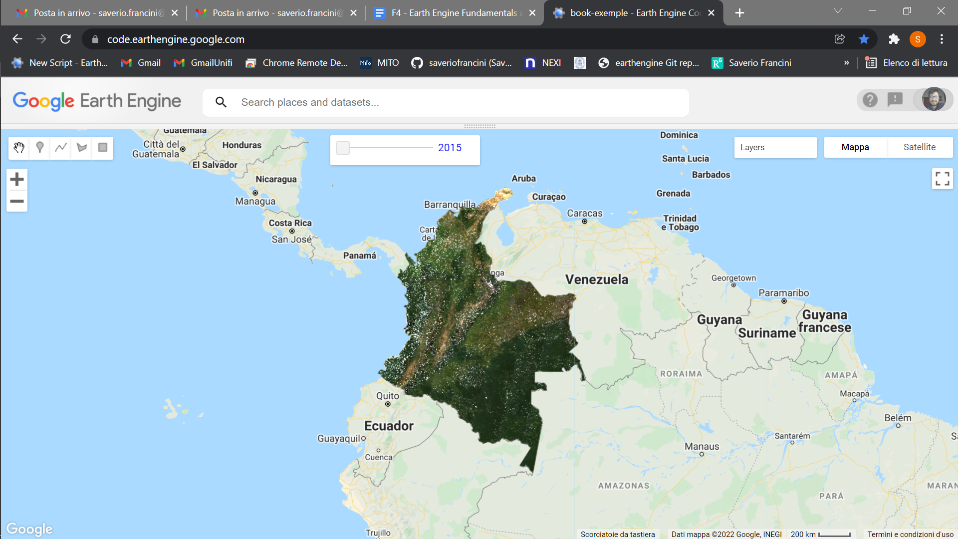
The first step is to define your AOI and center the map. The goal is to create a nationwide composite for the country of Colombia. We will use the Large Scale International Boundary (2017) simplified dataset from the US Department of State (USDOS), which contains polygons for all countries of the world.
// ---------- Section 1 ----------------- |
We will start creating a composite from the Landsat 8 collection. First, we define two time variables: startDate and endDate. Here, we will create a composite for the year 2019. Then, we will define a collection for the Landsat 8 Level 2, Collection 2, Tier 1 variable and filter it to our AOI and time period. We define and use a function to apply scaling factors to the Landsat 8 Collection 2 data.
// Define time variables. |
Now, we can create a composite. We will use the median function, which has the same effect as writing reduce(ee.Reducer.median()) as seen in Chap. F4.0, to reduce our ImageCollection to a median composite. Add the resulting composite to the map using visualization parameters.
// Create composite. |
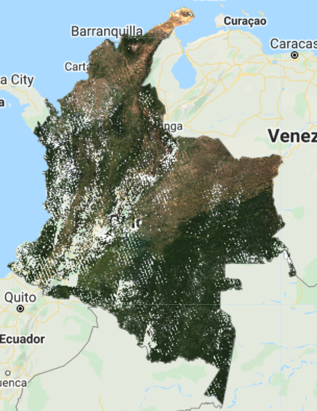
Fig. F4.3.1 Landsat 8 surface reflectance 2019 median composite of Colombia |

The resulting composite (Fig. F4.3.1) has lots of clouds, especially in the western, mountainous regions of Colombia. In tropical regions, it is very challenging to generate a high-quality, cloud-free composite without first filtering images for cloud cover, even if our collection is constrained to only include images acquired during the dry season. Therefore, let’s filter our collection by the CLOUD_COVER parameter to avoid cloudy images. We will start with images that have less than 50% cloud cover.
// Filter by the CLOUD_COVER property. |
Fig. F4.3.2 Landsat 8 surface reflectance 2019 median composite of Colombia filtered by cloud cover less than 50% |
This new composite (Fig. F4.3.2) looks slightly better than the previous one, but still very cloudy. Remember to turn off the first layer or adjust the transparency to visualize only this new composite. The code prints the size of these collections, using the size function) to see how many images were left out after we applied the cloud cover threshold. (There are 1201 images in the landsat8 collection, compared to 493 in the landsat8FiltClouds collection—a lot of scenes with cloud cover greater than or equal to 50%.)
Try adjusting the CLOUD_COVER threshold in the landsat8FiltClouds variable to different percentages and checking the results. For example, with 20% set as the threshold (Fig. F4.3.3), you can see that many parts of the country have image gaps. (Remember to turn off the first layer or adjust its transparency; you can also set the shown parameter in the Map.addLayer function to false so the layer does not automatically load). So there is a trade-off between a stricter cloud cover threshold and data availability. Additionally, even with a cloud filter, some tiles still present a large area cover of clouds.
Fig. F4.3.3 Landsat 8 surface reflectance 2019 median composite of Colombia filtered by cloud cover less than 20% |

This is due to persistent cloud cover in some regions of Colombia. However, a cloud mask can be applied to improve the results. The Landsat 8 Collection 2 contains a quality assessment (QA) band called QA_PIXEL that provides useful information on certain conditions within the data, and allows users to apply per-pixel filters. Each pixel in the QA band contains unsigned integers that represent bit-packed combinations of surface, atmospheric, and sensor conditions.
We will also make use of the QA_RADSAT band, which indicates which bands are radiometrically saturated. A pixel value of 1 means saturated, so we will be masking these pixels.
As described in Chap. F4.0, we will create a function to apply a cloud mask to an image, and then map this function over our collection. The mask is applied by using the updateMask function. This function “eliminates” undesired pixels from the analysis, i.e., makes them transparent, by taking the mask as the input. You will see that this cloud mask function (or similar versions) is used in other chapters of the book. Note: Remember to set the cloud cover threshold back to 50 in the landsat8FiltClouds variable.
// Define the cloud mask function. |
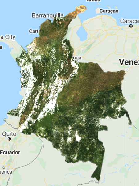
Fig. F4.3.4 Landsat 8 surface reflectance 2019 median composite of Colombia filtered by cloud cover less than 50% and with cloud mask applied |
Because we are dealing with bits, in the maskSrClouds function we utilized the bitwiseAnd and parseInt functions. These are functions that serve the purpose of unpacking the bit information. A bitwise AND is a binary operation that takes two equal-length binary representations and performs the logical AND operation on each pair of corresponding bits. Thus, if both bits in the compared positions have the value 1, the bit in the resulting binary representation is 1 (1 × 1=1); otherwise, the result is 0 (1 × 0=0 and 0 × 0=0). The parseInt function parses a string argument (in our case, five-character string '11111') and returns an integer of the specified numbering system, base 2.
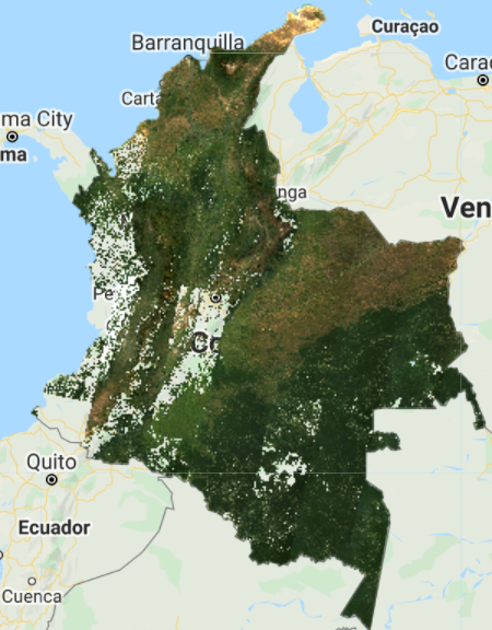
The resulting composite (Fig. F4.3.4) shows masked clouds, and is more spatially exhaustive in coverage compared to previous composites (don’t forget to uncheck the previous layers). This is because, when compositing all the images into one, we are not taking cloudy pixels into account anymore; therefore, the resulting pixel is not cloud covered but an actual representation of the landscape. However, data gaps are still an issue due to cloud cover. If you do not specifically need an annual composite, a first approach is to create a two-year composite to try to mitigate the missing data issue, or to have a series of rules that allows for selecting pixels for that particular year (as in Sect. 3 below). Change the startDate variable to 2018-01-01 to include all images from 2018 and 2019 in the collection. How does the cloud-masked composite (Fig. F4.3.5) compare to the 2019 one?
Fig. F4.3.5 One-year, startDate variable set to 2019-01-01, (left) and two-year, startDate variable set to 2018-01-01, (right) median composites with 50% cloud cover threshold and cloud mask applied |
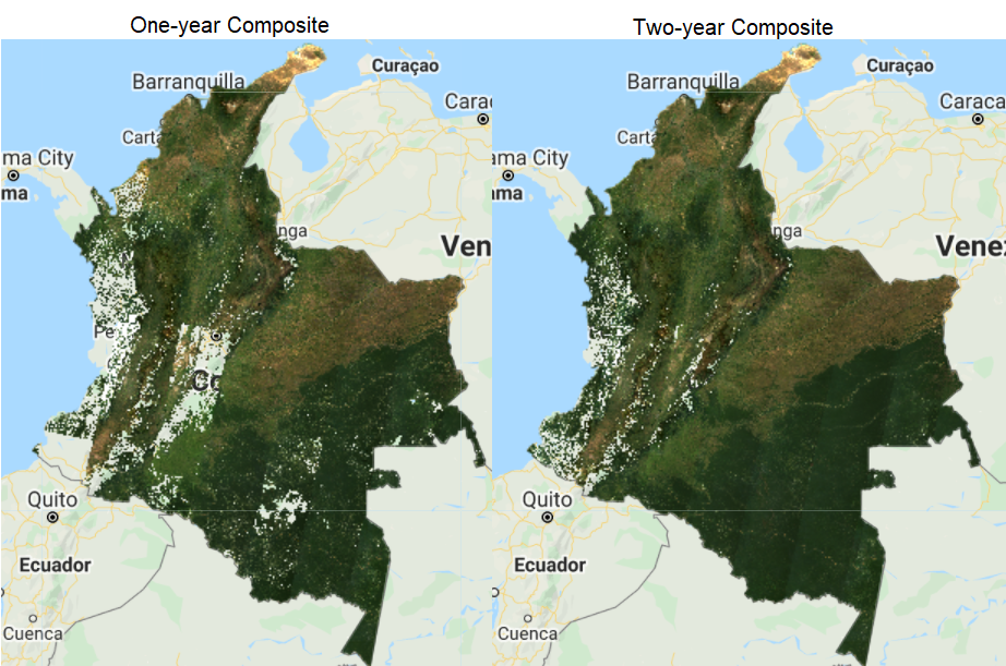
The resulting image has substantially fewer data gaps (you can zoom in to better see them). Again, if the time period is not a constraint for the creation of your composite, you can incorporate more images from a third year, and so on.
Code Checkpoint F43a. The book’s repository contains a script that shows what your code should look like at this point.
Section 2. Incorporating Data from Other Satellites
Another option to reduce the presence of data gaps in cloudy situations is to bring in imagery from other sensors acquired during the time period of interest. The Landsat collection spans multiple missions, which have continuously acquired uninterrupted data since 1972 at different acquisition dates. Next, we will try incorporating Landsat 7 Level 2, Collection 2, Tier 1 images from 2019 to fill the gaps in the 2019 Landsat 8 composite.
To generate a Landsat 7 composite, we apply similar steps to the ones we did for Landsat 8, so keep adding code to the same script from Sect. 1. First, define your Landsat 7 collection variable and the scaling function. Then, filter the collection, apply the cloud mask (since we know Colombia has persistent cloud cover), and apply the scaling function. Note that we will use the same cloud mask function defined above, since the bits information for Landsat 7 is the same as for Landsat 8. Finally, create the median composite. After pasting in the code below but before executing it, change the startDate variable back to 2019-01-01 in order to create a one-year composite of 2019.
// ---------- Section 2 ----------------- |
Fig. F4.3.6 One-year Landsat 7 median composite with 50% cloud cover threshold and cloud mask applied |
Note that we used bands: ['SR_B3', 'SR_B2', 'SR_B1'] to visualize the composite because Landsat 7 has different band designations. The sensors aboard each of the Landsat satellites were designed to acquire data in different ranges of frequencies along the electromagnetic spectrum. Whereas for Landsat 8, the red, green, and blue bands are B4, B3, and B2, respectively, for Landsat 7, these same bands are B3, B2, and B1, respectively.
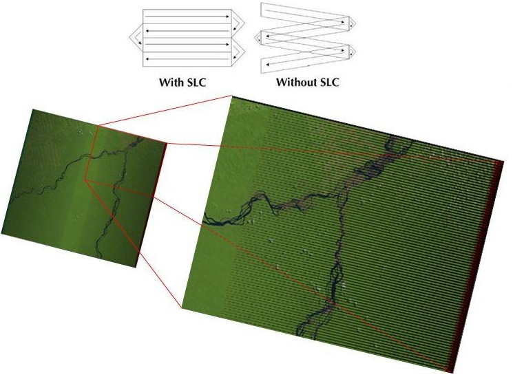
You should see an image with systematic gaps like the one shown in Fig. F4.3.6 (remember to turn off the other layers, and zoom in to better see the data gaps). Landsat 7 was launched in 1999, but since 2003, the sensor has acquired and delivered data with data gaps caused by a scan line corrector (SLC) failure. Without an operating SLC, the sensor’s line of sight traces a zig-zag pattern along the satellite ground track, and, as a result, the imaged area is duplicated and some areas are missed. When the Level 1 data are processed, the duplicated areas are removed, leaving data gaps (Fig. F4.3.7). For more information about Landsat 7 and SLC error, please refer to the USGS Landsat 7 page. However, even with the SLC error, we can still use the Landsat 7 data in our composite. Now, let’s combine the Landsat 7 and 8 collections.
Fig. F4.3.7 Landsat 7’s SLC-off condition. Source: USGS |
Since Landsat 7 and 8 have different band designations, first we create a function to rename the bands from Landsat 7 to match the names used for Landsat 8 and map that function over our Landsat 7 collection.
// Since Landsat 7 and 8 have different band designations, |
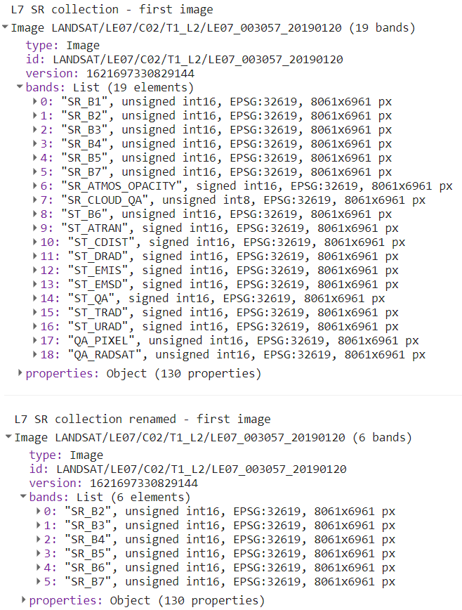
If you print the first images of both the landsat7FiltMasked and landsat7FiltMaskedRenamed collections (Fig. F4.3.8), you will see that the bands got renamed, and not all bands got copied over (SR_ATMOS_OPACITY, SR_CLOUD_QA, SR_B6, etc.). To copy these additional bands, simply add them to the rename function. You will need to rename SR_B6 so it does not have the same name as the new band 5.
Fig. F4.3.8 First images of landsat7FiltMasked and landsat7FiltMaskedRenamed, respectively |
Now we merge the two collections using the merge function for ImageCollection and mapping over a function to cast the Landsat 7 input values to a 32-bit float using the toFloat function for consistency. To merge collections, the number and names of the bands must be the same in each collection. We use the select function (Chap. F1.1) to select the Landsat 8 bands to be the same as Landsat 7’s. When creating the new Landsat 7 and 8 composite, if we did not select these 6 bands, we would get an error message for trying to composite a collection that has 6 bands (Landsat 7) with a collection that has 19 bands (Landsat 8).
// Merge Landsat collections. |
Now we have a collection with about 1000 images. Next, we will take the median of the values across the ImageCollection.
// Create Landsat 7 and 8 image composite and add to the Map. |
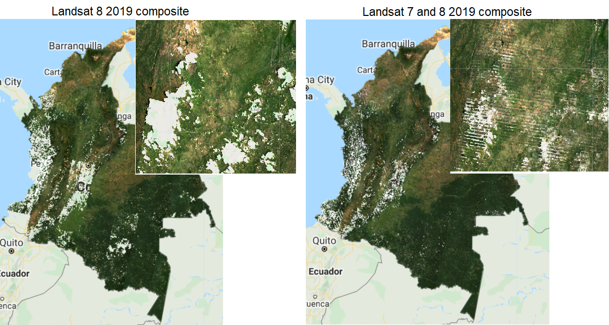
Comparing the composite generated considering both Landsat 7 and 8 to the Landsat 8-only composite, it is evident that there is a reduction in the amount of data gaps in the final result (Fig. F4.3.9). The resulting Landsat 7 and 8 image composite still has data gaps due to the presence of clouds and Landsat 7’s SLC-off data. You can try setting the center of the map to the point with latitude 3.6023 and longitude −75.0741 to see the inset example of Fig. F4.3.9.
Fig. F4.3.9 Landsat 8-only composite (left) and Landsat 7 and 8 composite (right) for 2019. Inset centered at latitude 3.6023, longitude −75.0741. |
Code Checkpoint F43b. The book’s repository contains a script that shows what your code should look like at this point.
Section 3. Best-Available-Pixel Compositing Earth Engine Application
This section presents an Earth Engine application that enables the generation of annual best-available-pixel (BAP) image composites by globally combining multiple Landsat sensors and images: GEE-BAP. Annual BAP image composites are generated by choosing optimal observations for each pixel from all available Landsat 5 TM, Landsat 7 ETM+, and Landsat 8 OLI imagery within a given year and within a given day range from a specified acquisition day of year, in addition to other constraints defined by the user. The data accessible via Earth Engine are from the USGS free and open archive of Landsat data. The Landsat images used are atmospherically corrected to surface reflectance values. Following White et al. (2014), a series of scoring functions ranks each pixel observation for (1) acquisition day of year, (2) cloud cover in the scene, (3) distance to clouds and cloud shadows, (4) presence of haze, and (5) acquisition sensor. Further information on the BAP image compositing approach can be found in Griffiths et al. (2013), and detailed information on tuning parameters can be found in White et al. (2014).
Code Checkpoint F43c. The book’s repository contains information about accessing the GEE-BAP interface and its related functions.
Fig. F4.3.10 GEE-BAP user interface controls |
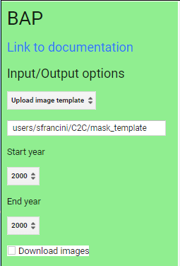
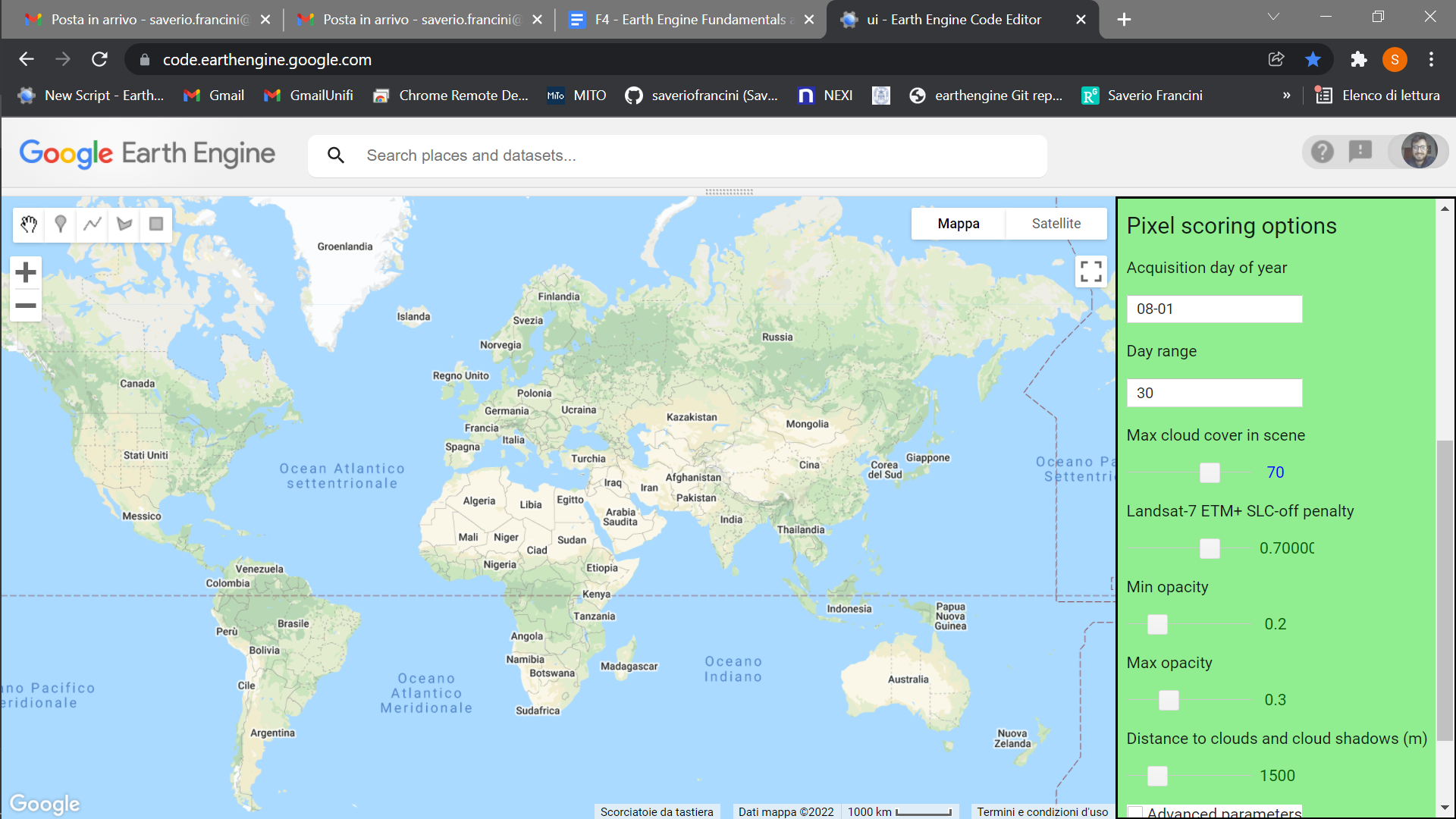
Once you have loaded the GEE-BAP interface (Fig. F4.3.10) using the instructions in the Code Checkpoint, you will notice that it is divided into three sections: (1) Input/Output options, (2) Pixel scoring options, and (3) Advanced parameters. Users indicate the study area, the time period for generating annual BAP composites (i.e., start and end years), and the path to store the results in the Input/Output options. Users have three options to define the study area. The Draw study area option uses the Draw a shape and Draw a rectangle tools to define the area of interest. The Upload image template option utilizes an image template uploaded by the user in TIFF format. This option is well suited to generating BAP composites that match the projection, pixel size, and extent to existing raster datasets. The Work globally option generates BAP composites for the entire globe; note that when this option is selected, complete data download is not available due to the Earth’s size. With Start year and End year, users can indicate the beginning and end of the annual time series of BAP image composites to be generated. Multiple image composites are then generated—one composite for each year—resulting in a time series of annual composites. For each year, composites are uniquely generated utilizing images acquired on the days within the specified Date range. Produced BAP composites can be saved in the indicated (Path) Google Drive folder using the Tasks tab. Results are generated in a tiled, TIFF format, accompanied by a CSV file that indicates the parameters used to construct the composite.
As noted, GEE-BAP implements five pixel scoring functions: (1) target acquisition day of year and day range, (2) maximum cloud coverage per scene, (3) distance to clouds and cloud shadows, (4) atmospheric opacity, and (5) a penalty for images acquired under the Landsat 7 ETM+ SLC-off malfunction. By defining the Acquisition day of year and Day range, those candidate pixels acquired closer to a defined acquisition day of year are ranked higher. Note that pixels acquired outside the day range window are excluded from subsequent composite development. For example, if the target day of year is defined as “08-01” and the day range as “31,” only those pixels acquired between July 1 and August 31 are considered, and the ones acquired closer to August 1 will receive a higher score.
The scoring function Max cloud cover in scene indicates the maximum percentage of cloud cover in an image that will be accepted by the user in the BAP image compositing process. Defining a value of 70% implies that only those scenes with less than or equal to 70% cloud cover will be considered as a candidate for compositing.
The Distance to clouds and cloud shadows scoring function enables the user to exclude those pixels identified to contain clouds and shadows by the QA mask from the generated BAP, as well as decreasing a pixel’s score if the pixel is within a specified proximity of a cloud or cloud shadow.
The Atmospheric opacity scoring function ranks pixels based on their atmospheric opacity values, which are indicative of hazy imagery. Pixels with opacity values that exceed a defined haze expectation (Max opacity) are excluded. Pixels with opacity values lower than a defined value (Min opacity) get the maximum score. Pixels with values in between these limits are scored following the functions defined by Griffiths et al. (2013). This scoring function is available only for Landsat 5 TM and Landsat 7 ETM+ imagery, which provides the opacity attribute in the image metadata file.
Finally, there is a Landsat 7 ETM+ SLC-off penalty scoring function that de-emphasizes images acquired following the ETM+ SLC-off malfunction in 2003. The aim of this scoring element is to ensure that TM or OLI data, which do not have stripes, take precedence over ETM+ when using dates after the SLC failure. This allows users to avoid the inclusion of multiple discontinuous small portions of images being used to produce the BAP image composites, thus reducing the spatial variability of the spectral data. The penalty applied to SLC-off imagery is defined directly proportional to the overall score. A large score reduces the chance that SLC-off imagery will be used in the composite. A value of 1 prevents SLC-off imagery from being used.
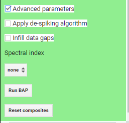
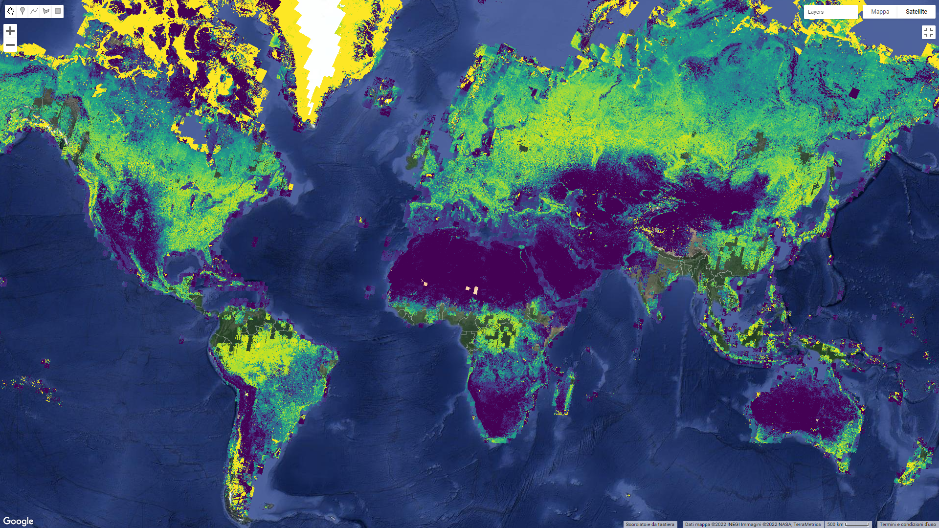
By default, the GEE-BAP application produces image composites using all the visible bands. The Spectral index option enables the user to produce selected spectral indices from the resulting BAP image composites. Available spectral indices include: Normalized Difference Vegetation Index (NDVI, Fig. F4.3.11), Enhanced Vegetation Index (EVI), and Normalized Burn Ratio (NBR), as well as several indices derived from the Tasseled Cap transformation: Wetness (TCW), Greenness (TCG), Brightness (TCB), and Angle (TCA). Composited indices are able to be downloaded as well as viewed on the map.
Fig. F4.3.11 Example of a global BAP image composite showing NDVI values generated using the GEE-BAP user interface |
GEE-BAP functions can be accessed programmatically, including pixel scoring parameters, as well as BAP image compositing (BAP), de-spiking (despikeCollection), data-gap infilling (infill), and displaying (ShowCollection) functions. The following code sets the scoring parameter values, then generates and displays the compositing results (Fig. F4.3.12) for a BAP composite that is de-spiked, with data gaps infilled using temporal interpolation. Copy and paste the code below into a new script.
// Define required parameters. |
Fig. F4.3.12 Outcome of the compositing code |
Code Checkpoint F43d. The book’s repository contains a script that shows what your code should look like at this point.
Synthesis
Assignment 1. Create composites for other cloudy regions or less cloudy regions. For example, change the country variable to 'Cambodia' or 'Mozambique'. Are more gaps present in the resulting composite? Can you change the compositing rules to improve this (using Acquisition day of year and Day range)? Different regions of the Earth have different cloud seasonal patterns, so the most appropriate date windows to acquire cloud-free composites will change depending on location. Also be aware that the larger the country, the longer it will take to generate the composite.
Assignment 2. Similarly, try creating composites for the wet and dry seasons of a region separately. Compare the two composites. Are some features brighter or darker? Is there evidence of drying of vegetation, such as related to leaf loss or reduction in herbaceous ground vegetation?
Assignment 3. Test different cloud threshold values and see if you can find an optimal threshold that balances data gaps against area coverage for your particular target date.
Conclusion
We cannot monitor what we cannot see. Image compositing algorithms provide robust and transparent tools to address issues with clouds, cloud shadows, haze, and smoke in remotely sensed images derived from optical satellite data, and expand data availability for remote sensing applications. The tools and approaches described here should provide you with some useful strategies to aid in mitigating the presence of cloud cover in your data. Note that the quality of image outcomes is a function of the quality of cloud masking routines applied to the source data to generate the various flags that are used in the scoring functions described herein. Different compositing parameters can be used to represent a given location as a function of conditions that are present at a given point in time and the information needs of the end user. Tuning or optimization of compositing parameters is possible (and recommended) to ensure best capture of the physical conditions of interest.
Feedback
To review this chapter and make suggestions or note any problems, please go now to bit.ly/EEFA-review. You can find summary statistics from past reviews at bit.ly/EEFA-reviews-stats.
References
Cloud-Based Remote Sensing with Google Earth Engine. (n.d.). CLOUD-BASED REMOTE SENSING WITH GOOGLE EARTH ENGINE. https://www.eefabook.org/
Cloud-Based Remote Sensing with Google Earth Engine. (2024). In Springer eBooks. https://doi.org/10.1007/978-3-031-26588-4
Braaten JD, Cohen WB, Yang Z (2015) Automated cloud and cloud shadow identification in Landsat MSS imagery for temperate ecosystems. Remote Sens Environ 169:128–138. https://doi.org/10.1016/j.rse.2015.08.006
Cao R, Chen Y, Chen J, et al (2020) Thick cloud removal in Landsat images based on autoregression of Landsat time-series data. Remote Sens Environ 249:112001. https://doi.org/10.1016/j.rse.2020.112001
Eberhardt IDR, Schultz B, Rizzi R, et al (2016) Cloud cover assessment for operational crop monitoring systems in tropical areas. Remote Sens 8:219. https://doi.org/10.3390/rs8030219
Griffiths P, van der Linden S, Kuemmerle T, Hostert P (2013) A pixel-based Landsat compositing algorithm for large area land cover mapping. IEEE J Sel Top Appl Earth Obs Remote Sens 6:2088–2101. https://doi.org/10.1109/JSTARS.2012.2228167
Hermosilla T, Wulder MA, White JC, Coops NC (2019) Prevalence of multiple forest disturbances and impact on vegetation regrowth from interannual Landsat time series (1985–2015). Remote Sens Environ 233:111403. https://doi.org/10.1016/j.rse.2019.111403
Hermosilla T, Wulder MA, White JC, et al (2015) An integrated Landsat time series protocol for change detection and generation of annual gap-free surface reflectance composites. Remote Sens Environ 158:220–234. https://doi.org/10.1016/j.rse.2014.11.005
Hermosilla T, Wulder MA, White JC, et al (2016) Mass data processing of time series Landsat imagery: Pixels to data products for forest monitoring. Int J Digit Earth 9:1035–1054. https://doi.org/10.1080/17538947.2016.1187673
Huang C, Thomas N, Goward SN, et al (2010) Automated masking of cloud and cloud shadow for forest change analysis using Landsat images. Int J Remote Sens 31:5449–5464. https://doi.org/10.1080/01431160903369642
Irish RR, Barker JL, Goward SN, Arvidson T (2006) Characterization of the Landsat-7 ETM+ automated cloud-cover assessment (ACCA) algorithm. Photogramm Eng Remote Sensing 72:1179–1188. https://doi.org/10.14358/PERS.72.10.1179
Kennedy RE, Yang Z, Cohen WB (2010) Detecting trends in forest disturbance and recovery using yearly Landsat time series: 1. LandTrendr - Temporal segmentation algorithms. Remote Sens Environ 114:2897–2910. https://doi.org/10.1016/j.rse.2010.07.008
Loveland TR, Dwyer JL (2012) Landsat: Building a strong future. Remote Sens Environ 122:22–29. https://doi.org/10.1016/j.rse.2011.09.022
Marshall GJ, Rees WG, Dowdeswell JA (1993) Limitations imposed by cloud cover on multitemporal visible band satellite data sets from polar regions. Ann Glaciol 17:113–120. https://doi.org/10.3189/S0260305500012696
Marshall GJ, Dowdeswell JA, Rees WG (1994) The spatial and temporal effect of cloud cover on the acquisition of high quality landsat imagery in the European Arctic sector. Remote Sens Environ 50:149–160. https://doi.org/10.1016/0034-4257(94)90041-8
Martins VS, Novo EMLM, Lyapustin A, et al (2018) Seasonal and interannual assessment of cloud cover and atmospheric constituents across the Amazon (2000–2015): Insights for remote sensing and climate analysis. ISPRS J Photogramm Remote Sens 145:309–327. https://doi.org/10.1016/j.isprsjprs.2018.05.013
Roberts D, Mueller N, McIntyre A (2017) High-dimensional pixel composites from Earth observation time series. IEEE Trans Geosci Remote Sens 55:6254–6264. https://doi.org/10.1109/TGRS.2017.2723896
Roy DP, Ju J, Kline K, et al (2010) Web-enabled Landsat data (WELD): Landsat ETM+ composited mosaics of the conterminous United States. Remote Sens Environ 114:35–49. https://doi.org/10.1016/j.rse.2009.08.011
Sano EE, Ferreira LG, Asner GP, Steinke ET (2007) Spatial and temporal probabilities of obtaining cloud-free Landsat images over the Brazilian tropical savanna. Int J Remote Sens 28:2739–2752. https://doi.org/10.1080/01431160600981517
White JC, Wulder MA, Hobart GW, et al (2014) Pixel-based image compositing for large-area dense time series applications and science. Can J Remote Sens 40:192–212. https://doi.org/10.1080/07038992.2014.945827
Zhu X, Helmer EH (2018) An automatic method for screening clouds and cloud shadows in optical satellite image time series in cloudy regions. Remote Sens Environ 214:135–153. https://doi.org/10.1016/j.rse.2018.05.024
Zhu Z, Wang S, Woodcock CE (2015) Improvement and expansion of the Fmask algorithm: Cloud, cloud shadow, and snow detection for Landsats 4–7, 8, and Sentinel 2 images. Remote Sens Environ 159:269–277. https://doi.org/10.1016/j.rse.2014.12.014Zhu Z, Woodcock CE (2014) Automated cloud, cloud shadow, and snow detection in multitemporal Landsat data: An algorithm designed specifically for monitoring land cover change. Remote Sens Environ 152:217–234. https://doi.org/10.1016/j.rse.2014.06.012
Zhu Z, Woodcock CE (2012) Object-based cloud and cloud shadow detection in Landsat imagery. Remote Sens Environ 118:83–94. https://doi.org/10.1016/j.rse.2011.10.028