Cloud-Based Remote Sensing with Google Earth Engine

Fundamentals and Applications

Part F3: Advanced Image Processing

Once you understand the basics of processing images in Earth Engine, this Part will present some of the more advanced processing tools available for treating individual images. These include creating regressions among image bands, transforming images with pixel-based and neighborhood-based techniques, and grouping individual pixels into objects that can then be classified.

Chapter F3.2: Neighborhood-Based Image Transformation

Authors

Karen Dyson, Andréa Puzzi Nicolau, David Saah, Nicholas Clinton

Overview

This chapter builds on image transformations to include a spatial component. All of these transformations leverage a neighborhood of multiple pixels around the focal pixel to inform the transformation of the focal pixel.

Learning Outcomes

• Performing image morphological operations.
• Defining kernels in Earth Engine.
• Applying kernels for image convolution to smooth and enhance images.
• Viewing a variety of neighborhood-based image transformations in Earth Engine.

Assumes you know how to:

• Import images and image collections, filter, and visualize (Part F1).
• Perform basic image analysis: select bands, compute indices, create masks, classify images (Part F2).

Github Code link for all tutorials

This code base is collection of codes that are freely available from different authors for google earth engine.

Github Source

Introduction to Theory

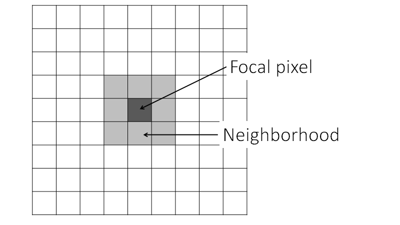
Neighborhood-based image transformations enable information from the pixels surrounding a focal pixel to inform the function transforming the value in the focal pixel (Fig. F3.2.1). For example, if your image has some pixels with outlier values, you can use a neighborhood-based transformation to diminish the effect of the outlier values (here we would recommend the median; see the Practicum section below). This is similar to how a moving average is performed (e.g., loess smoothing), but instead of averaging across one dimension (e.g., time), it averages across two dimensions (latitude and longitude).

Neighborhood-based image transformations are a foundational part of many remote sensing analysis workflows. For example, edge detection has been a critical part of land cover classification research efforts, including using Landsat 5 data in Minneapolis-St. Paul, Minnesota, USA (Stuckens et al. 2000), and using Landsat 7 and higher- resolution data including IKONOS in Accra, Ghana (Toure et al. 2018). Another type of neighborhood-based image transformation, the median operation, is an important part of remote sensing workflows due to its ability to dampen noise in images or classifications while maintaining edges (see ZhiYong et al. 2018, Lüttig et al. 2017). We will discuss these methods and others in this chapter.

Practicum

Section 1. Linear Convolution

If you have not already done so, be sure to add the book’s code repository to the Code Editor by entering https://code.earthengine.google.com/?accept_repo=projects/gee-edu/book into your browser. The book’s scripts will then be available in the script manager panel. If you have trouble finding the repo, you can visit this link for help.

Linear convolution refers to calculating a linear combination of pixel values in a neighborhood for the focal pixel (Fig. F3.2.1).

In Earth Engine, the neighborhood of a given pixel is specified by a kernel. The kernel defines the size and shape of the neighborhood and a weight for each position in the kernel. To implement linear convolution in Earth Engine, we’ll use the convolve with an ee.Kernel for the argument.

Convolving an image can be useful for extracting image information at different spatial frequencies.  For this reason, smoothing kernels are called low-pass filters (they let low-frequency data pass through) and edge-detection kernels are called high-pass filters. In the Earth Engine context, this use of the word “filter” is distinct from the filtering of image collections and feature collections seen throughout this book. In general in this book, filtering refers to retaining items in a set that have specified characteristics. In contrast, in this specific context of image convolution, “filter” is often used interchangeably with “kernel” when it is applied to the pixels of a single image. This chapter refers to these as “kernels” or “neighborhoods” wherever possible, but be aware of the distinction when you encounter the term “filter” in technical documentation elsewhere.  

Smoothing

A square kernel with uniform weights that sum to one is an example of a smoothing kernel. Using this kernel replaces the value of each pixel with the value of a summarizing function (usually, the mean) of its neighborhood. Because averages are less extreme than the values used to compute them, this tends to diminish image noise by replacing extreme values in individual pixels with a blend of surrounding values. When using a kernel to smooth an image in practice, the statistical properties of the data should be carefully considered (Vaiphasa 2006).

Let’s create and print a square kernel with uniform weights for our smoothing kernel.

Expand the kernel object in the Console to see the weights.  This kernel is defined by how many pixels it covers (i.e., radius is in units of pixels). Remember that your pixels may represent different real-world distances (spatial resolution is discussed in more detail in Chap. F1.3).

A kernel with radius defined in meters adjusts its size to an image’s pixel size, so you can't visualize its weights, but it's more flexible in terms of adapting to inputs of different spatial resolutions. In the next example, we will use kernels with radius defined in meters.

As first explored in Chap. F1.3, the National Agriculture Imagery Program (NAIP) is a GreatU.S. government program to acquire imagery over the continental United States using airborne sensors. The imagery has a spatial resolution of 0.5–2 m, depending on the state and the date collected.

Define a new point named point. We’ll locate it near the small town of Odessa in eastern Washington, USA. You can also search for “Odessa, WA, USA” in the search bar and define your own point.

Now filter and display the NAIP ImageCollection. For Washington state, there was NAIP imagery collected in 2018. We will use the reduce function in order to convert the image collection to an image for the convolution.

You’ll notice that the NAIP imagery selected with these operations covers only a very small area. This is because the NAIP image tiles are quite small, covering only a 3.75 x 3.75 minute quarter quadrangle plus a 300 m buffer on all four sides. For your own work using NAIP, you may want to use a rectangle or polygon to filter over a larger area and the reduce function instead of first.

Now define a kernel with a 2 m radius with uniform weights to use for smoothing.

Apply the smoothing operation by convolving the image with the kernel we’ve just defined.

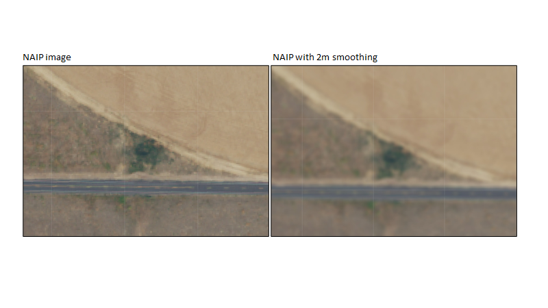
Now, compare the input image with the smoothed image. In Fig. F3.2.2, notice how sharp outlines around, for example, the patch of vegetation or the road stripes are less distinct.

To make the image even more smooth, you can increase the size of the neighborhood by increasing the pixel radius.

Gaussian Smoothing

A Gaussian kernel can also be used for smoothing. A Gaussian curve is also known as a bell curve. Think of convolving with a Gaussian kernel as computing the weighted average in each pixel's neighborhood, where closer pixels are weighted more heavily than pixels that are further away. Gaussian kernels preserve lines better than the smoothing kernel we just used, allowing them to be used when feature conservation is important, such as in detecting oil slicks (Wang and Hu 2015).

Now we’ll apply a Gaussian kernel to the same NAIP image.

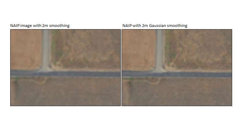
Pan and zoom around the NAIP image, switching between the two smoothing functions. Notice how the Gaussian smoothing preserves more of the detail of the image, such as the road lines and vegetation in Fig. F3.2.3.

Edge Detection

Edge-detection kernels are used to find rapid changes in remote sensing image values. These rapid changes usually signify edges of objects represented in the image data. Finding edges is useful for many applications, including identifying transitions between land cover and land use during classification.

A common edge-detection kernel is the Laplacian kernel. Other edge-detection kernels include the Sobel, Prewitt, and Roberts kernels. First, look at the Laplacian kernel weights:

Notice that if you sum all of the neighborhood values, the focal cell value is the negative of that sum. Now apply the kernel to our NAIP image and display the result:

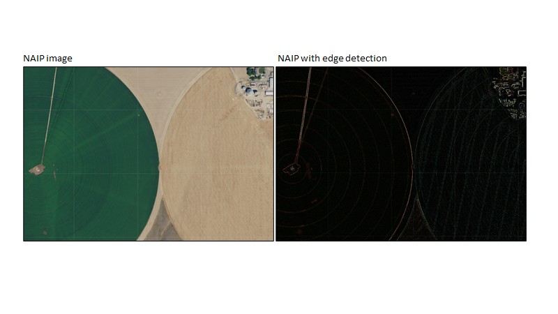
Edge-detection algorithms remove contrast within the image (e.g., between fields) and focus on the edge information (Fig. F3.2.4).

There are also algorithms in Earth Engine that perform edge detection. One of these is the Canny edge-detection algorithm (Canny 1986), which identifies the diagonal, vertical, and horizontal edges by using four separate kernels.

Sharpening

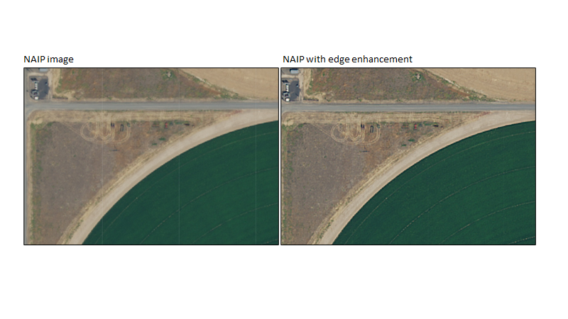
Image sharpening, also known as edge enhancement, leverages the edge-detection techniques we just explored to make the edges in an image sharper. This mimics the human eye’s ability to enhance separation between objects via Mach bands. To achieve this from a technical perspective, you add the image to the second derivative of the image.

To implement this in Earth Engine, we use a combination of Gaussian kernels through the Difference-of-Gaussians convolution (see Schowengerdt 2007 for details) and then add this to the input image. Start by creating two Gaussian kernels:

Next, combine the two Gaussian kernels into a Difference-of-Gaussians kernel and print the result:

Finally, apply the new kernel to the NAIP imagery with the convolve command, and then add the DoG convolved image to the original image with the add command (Fig. 3.2.5).

Code Checkpoint F32a. The book’s repository contains a script that shows what your code should look like at this point.

Section 2. Nonlinear Convolution

Where linear convolution functions involve calculating a linear combination of neighborhood pixel values for the focal pixel, nonlinear convolution functions use nonlinear combinations. Both linear and nonlinear convolution use the same concepts of the neighborhood, focal pixel, and kernel. The main difference from a practical standpoint is that nonlinear convolution approaches are implemented in Earth Engine using the reduceNeighborhood method on images.  

Median

Median neighborhood filters are used for denoising images. For example, some individual pixels in your image may have abnormally high or low values resulting from measurement error, sensor noise, or another cause. Using the mean operation described earlier to average values within a kernel would result in these extreme values polluting other pixels. That is, when a noisy pixel is present in the neighborhood of a focal pixel, the calculated mean will be pulled up or down due to that abnormally high- or low-value pixel. The median neighborhood filter can be used to minimize this issue. This approach is also useful because it preserves edges better than other smoothing approaches, an important feature for many types of classification.

Let’s reuse the uniform 5 x 5 kernel from above (uniformKernel) to implement a median neighborhood filter. As seen below, nonlinear convolution functions are implemented using reduceNeighborhood.

Inspect the median neighborhood filter map layer you’ve just added (Fig. F3.2.6). Notice how the edges are preserved instead of a uniform smoothing seen with the mean neighborhood filter. Look closely at features such as road intersections, field corners, and buildings.

Mode

The mode operation, which identifies the most commonly used number in a set, is particularly useful for categorical maps. Methods such as median and mean, which blend values found in a set, do not make sense for aggregating nominal data. Instead, we use the mode operation to get the value that occurs most frequently within each focal pixel’s neighborhood. The mode operation can be useful when you want to eliminate individual, rare pixel occurrences or small groups of pixels that are classified differently than their surroundings.

For this example, we will make a categorical map by thresholding the NIR band. First we will select the NIR band and then threshold it at 200 using the gt function (see also Chap. F2.0). Values higher than 200 will map to 1, while values equal to or below 200 will map to 0. We will then display the two classes as black and green. Thresholding the NIR band in this way is a very rough approximation of where vegetation occurs on the landscape, so we’ll call our layer veg.

Now use our uniform kernel to compute the mode in each 5 x 5 neighborhood.

The resulting image following the mode neighborhood filter has less individual pixel noise and more cohesive areas of vegetation (Fig. F3.2.7) .

Code Checkpoint F32b. The book’s repository contains a script that shows what your code should look like at this point.

Section 3. Morphological Processing

The idea of morphology is tied to the concept of objects in images. For example, suppose the patches of 1s in the veg image from the previous section represent patches of vegetation. Morphological processing helps define these objects so that the processed images can better inform classification processes, such as object-based classification (Chap. F3.3), and as a post-processing approach to reduce noise caused by the classification process. Below are four of the most important morphological processing approaches.

Dilation

If the classification underestimates the actual distribution of vegetation and contains “holes,” a max operation can be applied across the neighborhood to expand the areas of vegetation. This process is known as a dilation (Fig. F3.2.8).

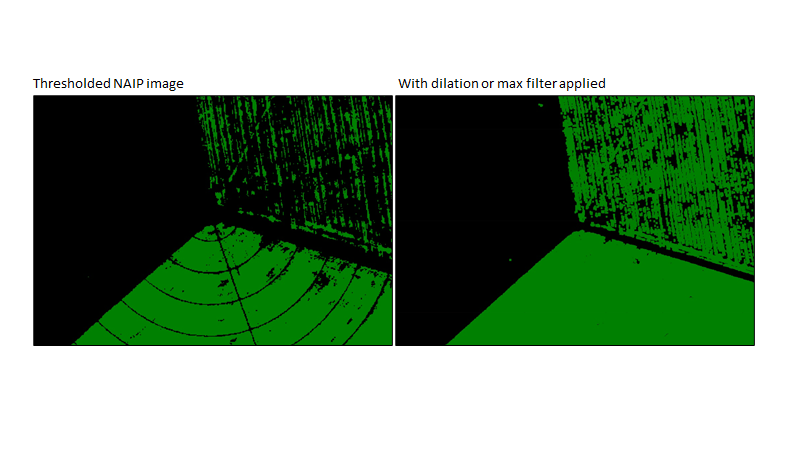
To explore the effects of dilation, you might try to increase the size of the kernel (i.e., increase the radius), or to apply reduceNeighborhood repeatedly. There are shortcuts in the API for some common reduceNeighborhood actions, including focalMax and focalMin, for example.

Erosion

The opposite of dilation is erosion, for decreasing the size of the patches. To effect an erosion, a min operation can be applied to the values inside the kernel as each pixel is evaluated.

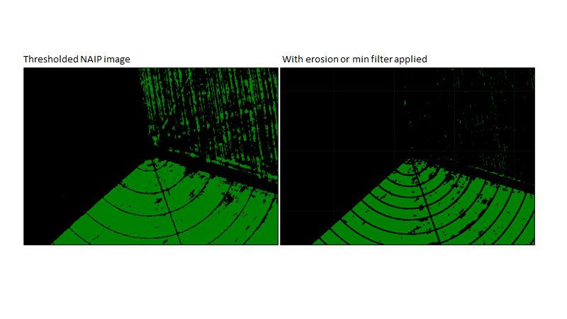
Carefully inspect the result compared to the input (Fig. F3.2.9). Note that the shape of the kernel affects the shape of the eroded patches (the same effect occurs in the dilation). Because we used a square kernel, the eroded patches and dilated areas are square. You can explore this effect by testing kernels of different shapes.  

As with the dilation, note that you can get more erosion by increasing the size of the kernel or applying the operation more than once.

Opening 

To remove small patches of green that may be unwanted, we will perform an erosion followed by a dilation. This process is called opening, and works to delete small details and is useful for removing noise. We can use our eroded image and perform a dilation on it (Fig. F3.2.10).

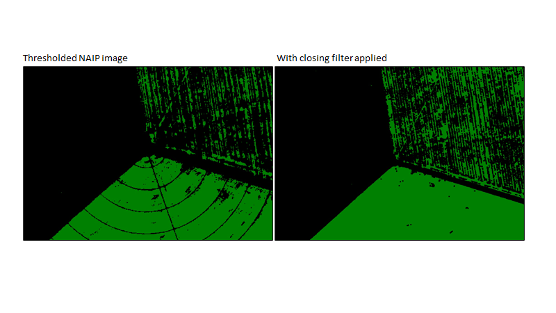
Closing

Finally, the opposite of opening is closing, which is a dilation operation followed by an erosion. This series of transformations is used to remove small holes in the input patches (Fig. F3.2.11).

Closely examine the difference between each morphological operation and the veg input. You can adjust the effect of these morphological operators by adjusting the size and shape of the kernel (also called a “structuring element” in this context, because of its effect on the spatial structure of the result), or applying the operations repeatedly. When used for post-processing of, for example, a classification output, this process will usually require multiple iterations to balance accuracy with class cohesion.

Code Checkpoint F32c. The book’s repository contains a script that shows what your code should look like at this point.

Section 4. Texture

The final group of neighborhood-based operations we’ll discuss are meant to detect or enhance the “texture” of the image. Texture measures use a potentially complex, usually nonlinear calculation using the pixel values within a neighborhood. From a practical perspective, texture is one of the cues we use (often unconsciously) when looking at a remote sensing image in order to identify features. Some examples include distinguishing tree cover, examining the type of canopy cover, and distinguishing crops. Measures of texture may be used on their own, or may be useful as inputs to regression, classification, and other analyses when they help distinguish between different types of land cover/land use or other features on the landscape.

There are many ways to assess texture in an image, and a variety of functions have been implemented to compute texture in Earth Engine. 

Standard Deviation

The standard deviation (SD) measures the spread of the distribution of image values in the neighborhood. A textureless neighborhood, in which there is only one value within the neighborhood, has a standard deviation of 0. A neighborhood with significant texture will have a high standard deviation, the value of which will be influenced by the magnitude of the values within the neighborhood.

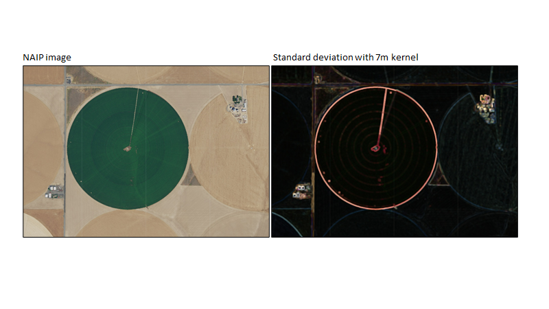
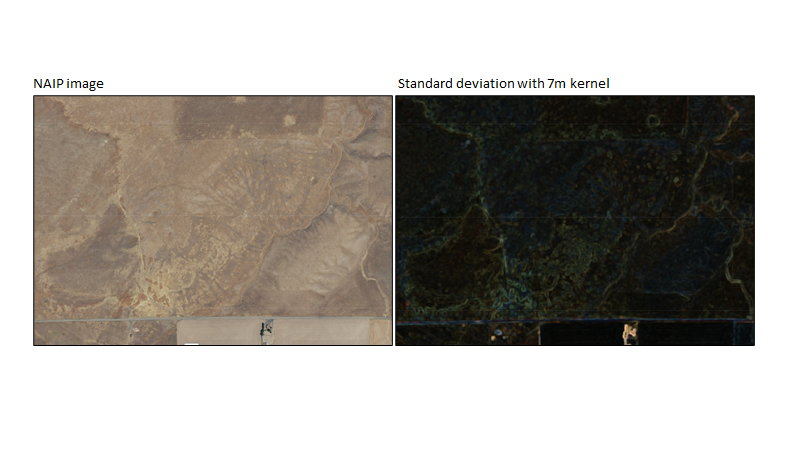
Compute neighborhood SD for the NAIP image by first defining a 7 m radius kernel, and then using the stdDev reducer with the kernel.

The resulting image for our fields somewhat resembles the image for edge detection (Fig. F3.2.12).

You can pan around the example area to find buildings or pasture land and examine these features. Notice how local variation and features appear, such as the washes (texture variation caused by water) in Fig. F3.2.13.

Entropy

For discrete valued inputs, you can compute entropy in a neighborhood. Broadly, entropy is a concept of disorder or randomness. In this case, entropy is an index of the numerical diversity in the neighborhood.

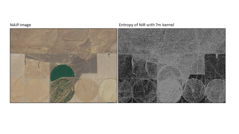
We’ll compute entropy using the entropy function in Earth Engine and our bigKernel structuring element. Notice that if you try to run the entropy on the entire NAIP image (imageNAIP), you will get an error that only 32-bit or smaller integer types are currently supported. So, let’s cast the image to contain an integer in every pixel using the int function. We’ll operate on the near-infrared band since it is important for vegetation.

The resulting entropy image has low values where the 7 m neighborhood around a pixel is homogeneous, and high values where the neighborhood is heterogeneous (Fig. F3.2.14).

Gray-level Co-occurrence Matrices 

The gray-level co-occurrence matrix (GLCM) is based on gray-scale images. It evaluates the co-occurrence of similar values occurring horizontally, vertically, or diagonally. More formally, the GLCM is computed by forming an M x M matrix for an image with M possible DN values, then computing entry i,j as the frequency at which DN=i is adjacent to DN=j. In other words, the matrix represents the relationship between two adjacent pixels.

Once the GLCM has been calculated, a variety of texture metrics can be computed based on that matrix. One of these is contrast. To do this, we first use the glcmTexture function. This function computes 14 original GLCM metrics (Haralick et al. 1973) and four later GLCM metrics (Conners et al.1984). The glcmTexture function creates an image where each band is a different metric. Note that the input needs to be an integer, so we’ll use the same integer NAIP layer as above, and we need to provide a size for the neighborhood (here it is 7).

Now let’s display the contrast results for the red, green, and blue bands. Contrast is the second band, and measures the local contrast of an image.

The resulting image highlights where there are differences in the contrast. For example, in Fig. F3.2.15, we can see that the red band has high contrast within this patchy field.

Spatial Statistics

Spatial statistics describe the distribution of different events across space, and are extremely useful for remote sensing (Stein et al. 1998). Uses include anomaly detection, topographical analysis including terrain segmentation, and texture analysis using spatial association, which is how we will use it here. Two interesting texture measures from the field of spatial statistics include local Moran's I and local Geary's C (Anselin 1995).

To compute a local Geary's C with the NAIP image as input, first create a 9 x 9 kernel and then calculate local Geary’s C.

Now that we have a kernel, we can calculate the maximum of the four NAIP bands and use this with the kernel to calculate local Geary’s C. There is no built-in function for Geary’s C in Earth Engine, so we create our own using the subtract, pow (power), sum, and divide functions (Chap. F3.1).

Inspecting the resulting layer shows that boundaries between fields, building outlines, and roads have high values of Geary’s C. This makes sense because across bands there will be high spatial autocorrelation within fields that are homogenous, whereas between fields (at the field boundary) the area will be highly heterogeneous (Fig. F3.2.16).

Code Checkpoint F32d. The book’s repository contains a script that shows what your code should look like at this point.

Synthesis

In this chapter we have explored many different neighborhood-based image transformations. These transformations have practical applications for remote sensing image analysis. Using transformation, you can use what you have learned in this chapter and in F2.1 to:

• Use raw imagery (red, green, blue, and near-infrared bands) to create an image classification.
• Use neighborhood transformations to create input imagery for an image classification and run the image classification.
• Use one or more of the morphological transformations to clean up your image classification.

Assignment 1. Compare and contrast your image classifications when using raw imagery compared with using neighborhood transformations.

Assignment 2. Compare and contrast your unaltered image classification and your image classification following morphological transformations.

Conclusion

Neighborhood-based image transformations enable you to extract information about each pixel’s neighborhood to perform multiple important operations. Among the most important are smoothing, edge detection and definition, morphological processing, texture analysis, and spatial analysis. These transformations are a foundational part of many larger remote sensing analysis workflows. They may be used as imagery pre-processing steps and as individual layers in regression and classifications, to inform change detection, and for other purposes.

Feedback

To review this chapter and make suggestions or note any problems, please go now to bit.ly/EEFA-review. You can find summary statistics from past reviews at bit.ly/EEFA-reviews-stats.

References

Cloud-Based Remote Sensing with Google Earth Engine. (n.d.). CLOUD-BASED REMOTE SENSING WITH GOOGLE EARTH ENGINE. https://www.eefabook.org/

Cloud-Based Remote Sensing with Google Earth Engine. (2024). In Springer eBooks. https://doi.org/10.1007/978-3-031-26588-4

Anselin L (1995) Local indicators of spatial association—LISA. Geogr Anal 27:93–115. https://doi.org/10.1111/j.1538-4632.1995.tb00338.x

Canny J (1986) A computational approach to edge detection. IEEE Trans Pattern Anal Mach Intell PAMI-8:679–698. https://doi.org/10.1109/TPAMI.1986.4767851

Castleman KR (1996) Digital Image Processing. Prentice Hall Press

Conners RW, Trivedi MM, Harlow CA (1984) Segmentation of a high-resolution urban scene using texture operators. Comput Vision, Graph Image Process 25:273–310. https://doi.org/10.1016/0734-189X(84)90197-X

Haralick RM, Dinstein I, Shanmugam K (1973) Textural features for image classification. IEEE Trans Syst Man Cybern SMC-3:610–621. https://doi.org/10.1109/TSMC.1973.4309314

Lüttig C, Neckel N, Humbert A (2017) A combined approach for filtering ice surface velocity fields derived from remote sensing methods. Remote Sens 9:1062. https://doi.org/10.3390/rs9101062

Schowengerdt RA (2006) Remote Sensing: Models and Methods for Image Processing. Elsevier

Stein A, Bastiaanssen WGM, De Bruin S, et al (1998) Integrating spatial statistics and remote sensing. Int J Remote Sens 19:1793–1814. https://doi.org/10.1080/014311698215252

Stuckens J, Coppin PR, Bauer ME (2000) Integrating contextual information with per-pixel classification for improved land cover classification. Remote Sens Environ 71:282–296. https://doi.org/10.1016/S0034-4257(99)00083-8

Toure SI, Stow DA, Shih H-C, et al (2018) Land cover and land use change analysis using multi-spatial resolution data and object-based image analysis. Remote Sens Environ 210:259–268. https://doi.org/10.1016/j.rse.2018.03.023

Vaiphasa C (2006) Consideration of smoothing techniques for hyperspectral remote sensing. ISPRS J Photogramm Remote Sens 60:91–99. https://doi.org/10.1016/j.isprsjprs.2005.11.002

Wang M, Hu C (2015) Extracting oil slick features from VIIRS nighttime imagery using a Gaussian filter and morphological constraints. IEEE Geosci Remote Sens Lett 12:2051–2055. https://doi.org/10.1109/LGRS.2015.2444871

ZhiYong L, Shi W, Benediktsson JA, Gao L (2018) A modified mean filter for improving the classification performance of very high-resolution remote-sensing imagery. Int J Remote Sens 39:770–785. https://doi.org/10.1080/01431161.2017.1390275