Cloud-Based Remote Sensing with Google Earth Engine
Fundamentals and Applications

Part F4: Interpreting Image Series
One of the paradigm-changing features of Earth Engine is the ability to access decades of imagery without the previous limitation of needing to download all the data to a local disk for processing. Because remote-sensing data files can be enormous, this used to limit many projects to viewing two or three images from different periods. With Earth Engine, users can access tens or hundreds of thousands of images to understand the status of places across decades.
Chapter F4.2: Aggregating Images for Time Series
Author
Ujaval Gandhi
Overview
Many remote sensing datasets consist of repeated observations over time. The interval between observations can vary widely. The Global Precipitation Measurement dataset, for example, produces observations of rain and snow worldwide every three hours. The Climate Hazards Group InfraRed Precipitation with Station (CHIRPS) project produces a gridded global dataset at the daily level and also for each five-day period. The Landsat 8 mission produces a new scene of each location on Earth every 16 days. With its constellation of two satellites, the Sentinel-2 mission images every location every five days.
Many applications, however, require computing aggregations of data at time intervals different from those at which the datasets were produced. For example, for determining rainfall anomalies, it is useful to compare monthly rainfall against a long-period monthly average.
While individual scenes are informative, many days are cloudy, and it is useful to build a robust cloud-free time series for many applications. Producing less cloudy or even cloud-free composites can be done by aggregating data to form monthly, seasonal, or yearly composites built from individual scenes. For example, if you are interested in detecting long-term changes in an urban landscape, creating yearly median composites can enable you to detect change patterns across long time intervals with less worry about day-to-day noise.
This chapter will cover the techniques for aggregating individual images from a time series at a chosen interval. We will take the CHIRPS time series of rainfall for one year and aggregate it to create a monthly rainfall time series.
Learning Outcomes
- Using the Earth Engine API to work with dates.
- Aggregating values from an ImageCollection to calculate monthly, seasonal, or yearly images.
- Plotting the aggregated time series at a given location.
Assumes you know how to:
- Import images and image collections, filter, and visualize (Part F1).
- Create a graph using ui.Chart (Chap. F1.3).
- Write a function and map it over an ImageCollection (Chap. F4.0).
- Summarize an ImageCollection with reducers (Chap. F4.0, Chap. F4.1).
- Inspect an Image and an ImageCollection, as well as their properties (Chap. F4.1).
Github Code link for all tutorials
This code base is collection of codes that are freely available from different authors for google earth engine.
Introduction to Theory
CHIRPS is a high-resolution global gridded rainfall dataset that combines satellite-measured precipitation with ground station data in a consistent, long time-series dataset. The data are provided by the University of California, Santa Barbara, and are available from 1981 to the present. This dataset is extremely useful in drought monitoring and assessing global environmental change over land. The satellite data are calibrated with ground station observations to create the final product.
In this exercise, we will work with the CHIRPS dataset using the pentad. A pentad represents the grouping of five days. There are six pentads in a calendar month, with five pentads of exactly five days each and one pentad with the remaining three to six days of the month. Pentads reset at the beginning of each month, and the first day of every month is the start of a new pentad. Values at a given pixel in the CHIRPS dataset represent the total precipitation in millimeters over the pentad.
Practicum
Section 1. Filtering an Image Collection
We will start by accessing the CHIRPS Pentad collection and filtering it to create a time series for a single year.
var chirps=ee.ImageCollection('UCSB-CHG/CHIRPS/PENTAD'); |
The CHIRPS collection contains one image for every pentad. The filtered collection above is filtered to contain one year, which equates to 72 global images. If you expand the printed collection in the Console, you will be able to see the metadata for individual images; note that their date stamps indicate that they are spaced evenly every five days (Fig. F4.2.1).
Fig. F4.2.1 CHIRPS time series for one year |
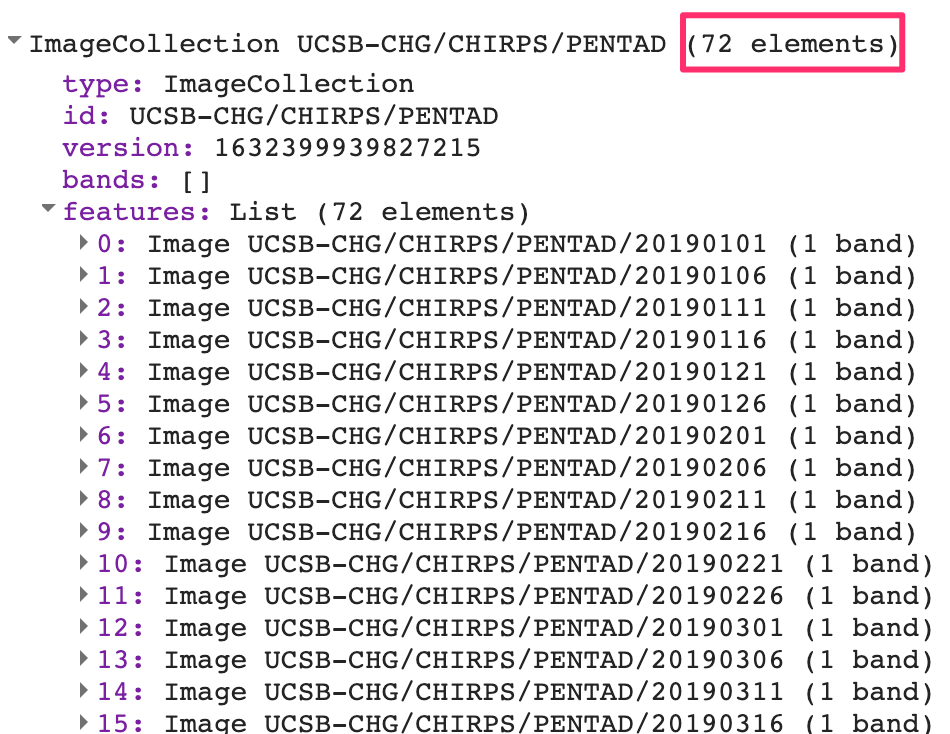
Each image’s pixel values store the total precipitation during the pentad. Without aggregation to a period that matches other datasets, these layers are not very useful. For hydrological analysis, we typically need the total precipitation for each month or for a season. Let’s aggregate this collection so that we have 12 images—one image per month, with pixel values that represent the total precipitation for that month.
Code Checkpoint F42a. The book’s repository contains a script that shows what your code should look like at this point.
Section 2. Working with Dates
To aggregate the time series, we need to learn how to create and manipulate dates programmatically. This section covers some functions from the ee.Date module that will be useful.
The Earth Engine API has a function called ee.Date.fromYMD that is designed to create a date object from year, month, and day values. The following code snippet shows how to define a variable containing the year value and create a date object from it. Paste the following code in a new script:
var chirps=ee.ImageCollection('UCSB-CHG/CHIRPS/PENTAD'); |
Now, let’s determine how to create an end date in order to be able to specify a desired time interval. The preferred way to create a date relative to another date is using the advance function. It takes two parameters—a delta value and the unit of time—and returns a new date. The code below shows how to create a date one year in the future from a given date. Paste it into your script.
var endDate=startDate.advance(1, 'year'); |
Next, paste the code below to perform filtering of the CHIRPS data using these calculated dates. After running it, check that you had accurately set the dates by looking for the dates of the images inside the printed result..
var yearFiltered=chirps |
Another date function that is very commonly used across Earth Engine is millis. This function takes a date object and returns the number of milliseconds since the arbitrary reference date of the start of the year 1970: 1970-01-01T00:00:00Z. This is known as the “Unix Timestamp”; it is a standard way to convert dates to numbers and allows for easy comparison between dates with high precision. Earth Engine objects store the timestamps for images and features in special properties called system:time_start and system:time_end. Both of these properties need to be supplied with a number instead of dates, and the millis function can help you do that. You can print the result of calling this function and check for yourself.
print(startDate, 'Start date'); |
We will use the millis function in the next section when we need to set the system:time_start and system:time_end properties of the aggregated images.
Code Checkpoint F42b. The book’s repository contains a script that shows what your code should look like at this point.
Section 3. Aggregating Images
Now we can start aggregating the pentads into monthly sums. The process of aggregation has two fundamental steps. The first is to determine the beginning and ending dates of one time interval (in this case, one month), and the second is to sum up all of the values (in this case, the pentads) that fall within each interval. To begin, we can envision that the resulting series will contain 12 images. To prepare to create an image for each month, we create an ee.List of values from 1 to 12. We can use the ee.List.sequence function, as first presented in Chap. F1.0, to create the list of items of type ee.Number. Continuing with the script of the previous section, paste the following code:
// Aggregate this time series to compute monthly images. |
Next, we write a function that takes a single month as the input and returns an aggregated image for that month. Given beginningMonth as an input parameter, we first create a start and end date for that month based on the year and month variables. Then we filter the collection to find all images for that month. To create a monthly precipitation image, we apply ee.Reducer.sum to reduce the six pentad images for a month to a single image holding the summed value across the pentads. We also expressly set the timestamp properties system:time_start and system:time_end of the resulting summed image. We can also set year and month, which will help us filter the resulting collection later.
// Write a function that takes a month number |
We now have an ee.List containing items of type ee.Number from 1 to 12, with a function that can compute a monthly aggregated image for each month number. All that is left to do is to map the function over the list. As described in Chaps. F4.0 and F4.1, the map function passes over each image in the list and runs createMonthlyImage. The function first receives the number “1” and executes, returning an image to Earth Engine. Then it runs on the number “2”, and so on for all 12 numbers. The result is a list of monthly images for each month of the year.
// map() the function on the list of months |
We can create an ImageCollection from this ee.List of images using the ee.ImageCollection.fromImages function.
// Create an ee.ImageCollection. |
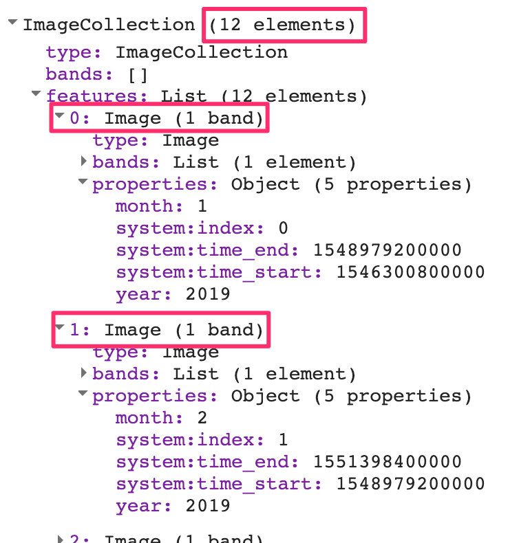
We have now successfully computed an aggregated collection from the source ImageCollection by filtering, mapping, and reducing, as described in Chaps. F4.0 and F4.1. Expand the printed collection in the Console and you can verify that we now have 12 images in the newly created ImageCollection (Fig. F4.2.2).
Fig. F4.2.2 Aggregated time series |
Code Checkpoint F42c. The book’s repository contains a script that shows what your code should look like at this point.
Section 4. Plotting Time Series
One useful application of gridded precipitation datasets is to analyze rainfall patterns. We can plot a time-series chart for a location using the newly computed time series. We can plot the pixel value at any given point or polygon. Here we create a point geometry for a given coordinate. Continuing with the script of the previous section, paste the following code:
// Create a point with coordinates for the city of Bengaluru, India. |
Earth Engine comes with a built-in ui.Chart.image.series function that can plot time series. In addition to the imageCollection and region parameters, we need to supply a scale value. The CHIRPS data catalog page indicates that the resolution of the data is 5566 meters, so we can use that as the scale. The resulting chart is printed in the Console.
var chart=ui.Chart.image.series({ |
We can make the chart more informative by adding axis labels and a title. The setOptions function allows us to customize the chart using parameters from Google Charts. To customize the chart, paste the code below at the bottom of your script. The effect will be to see two charts in the editor: one with the old view of the data, and one with the customized chart.
var chart=ui.Chart.image.series({ |
The customized chart (Fig. F4.2.3) shows the typical rainfall pattern in the city of Bengaluru, India. Bengaluru has a temperate climate, with pre-monsoon rains in April and May cooling down the city and a moderate monsoon season lasting from June to September.
Fig. F4.2.3 Monthly rainfall chart |

Code Checkpoint F42d. The book’s repository contains a script that shows what your code should look like at this point.
Synthesis
Assignment 1. The CHIRPS collection contains data for 40 years. Aggregate the same collection to yearly images and create a chart for annual precipitation from 1981 to 2021 at your chosen location.
Instead of creating a list of months and writing a function to create monthly images, we will create a list of years and write a function to create yearly images. The code snippet below will help you get started.
var chirps=ee.ImageCollection('UCSB-CHG/CHIRPS/PENTAD'); |
Conclusion
In this chapter, you learned how to aggregate a collection to months and plot the resulting time series for a location. This chapter also introduced useful functions for working with the dates that will be used across many different applications. You also learned how to iterate over a list using the map function. The technique of mapping a function over a list or collection is essential for processing data. Mastering this technique will allow you to scale your analysis using the parallel computing capabilities of Earth Engine.
Feedback
To review this chapter and make suggestions or note any problems, please go now to bit.ly/EEFA-review. You can find summary statistics from past reviews at bit.ly/EEFA-reviews-stats.
References
Cloud-Based Remote Sensing with Google Earth Engine. (n.d.). CLOUD-BASED REMOTE SENSING WITH GOOGLE EARTH ENGINE. https://www.eefabook.org/
Cloud-Based Remote Sensing with Google Earth Engine. (2024). In Springer eBooks. https://doi.org/10.1007/978-3-031-26588-4
Banerjee A, Chen R, Meadows ME, et al (2020) An analysis of long-term rainfall trends and variability in the Uttarakhand Himalaya using Google Earth Engine. Remote Sens 12:709. https://doi.org/10.3390/rs12040709
Funk C, Peterson P, Landsfeld M, et al (2015) The climate hazards infrared precipitation with stations – a new environmental record for monitoring extremes. Sci Data 2:1–21. https://doi.org/10.1038/sdata.2015.66
Okamoto K, Ushio T, Iguchi T, et al (2005) The global satellite mapping of precipitation (GSMaP) project. In: International Geoscience and Remote Sensing Symposium (IGARSS). pp 3414–3416