Cloud-Based Remote Sensing with Google Earth Engine

Fundamentals and Applications

Part A3: Terrestrial Applications

Earth’s terrestrial surface is analyzed regularly by satellites, in search of both change and stability. These are of great interest to a wide cross-section of Earth Engine users, and projects across large areas illustrate both the challenges and opportunities for life on Earth. Chapters in this Part illustrate the use of Earth Engine for disturbance, understanding long-term changes of rangelands, and creating optimum study sites.

Chapter A3.2: Mangroves

Author

Aurélie Shapiro

Overview

Mangrove ecosystems are tropical coastal forests that are adapted to saltwater environments. Their unique qualities of existing primarily in moist environments at low elevation along shorelines, lack of seasonality, and compact pattern make them relatively easy to identify in satellite images. In this chapter we present a series of automated steps, including water masking, to extract mangroves from a fusion of optical and active radar data. Furthermore, as global mangrove datasets are readily available in Google Earth Engine, we present an approach to automatically extract training data from existing information, saving time and effort in your supervised classification. The method can then be adapted to create subsequent maps from your own results to produce changes in mangrove ecosystems over time.    

Learning Outcomes

• Fusing Sentinel-1 and -2 optical/radar sensors.
• Sampling points on an image to create training and testing datasets.
• Calculating additional indices to add to the image stack.
• Applying an automatic water masking function and buffering to focus classification on coastal areas likely to have mangroves.
• Understanding supervised classification with random forests using automatically derived training data.
• Evaluating training and model accuracy.

Helps if you know how to:

• Import images and image collections, filter, and visualize (Part F1).
• Perform basic image analysis: select bands, compute indices, create masks (Part F2).
• Perform pixel-based supervised or unsupervised classification (Chap. F2.1).
• Use expressions to perform calculations on image bands (Chap. F3.1).
• Perform image morphological operations (Chap. F3.2).
• Create or access image mosaics (Chap. F4.3).
• Interpret Otsu’s method for partitioning a histogram (Chap. A2.3).

Github Code link for all tutorials

This code base is collection of codes that are freely available from different authors for google earth engine.

Github Source

Introduction to Theory

Mangrove ecosystems are highly productive environments that provide essential services, notably the storage of blue carbon, stabilization and protection of coastlines from storms and coastal events, and the provision of nurseries for fish. Mangrove ecosystems also enhance associated coral reef ecosystems, which are crucial to supporting local livelihoods (Bryan-Brown et al. 2020). Mangrove forests consist of specialized species adapted to saltwater environments located in tropical and subtropical latitudes. Over 1.3 billion people live in tropical coastal areas and rely on mangrove ecosystems for their health, safety, and livelihood. It is important to map, monitor, and quantify their change over time in order to properly conserve and restore them.

In this chapter, we will review the basic process for mapping mangroves using Sentinel-1 and -2 imagery. Mangroves are particularly recognizable in satellite imagery by their wetness—these ecosystems thrive at the water/land interface, making them easy to distinguish with satellite sensors that are sensitive to vegetation and water. We use sensor fusion to combine the advantages of multiple sensor types. For optical data, we extract relevant vegetation and water indices to discern mangroves, and we use active radar data for its capacity to detect water and derive canopy texture information.

In this chapter, we will show you how to evaluate mangroves at 10 m resolution using a fusion of optical and radar sensors (Sentinel-1 and -2) and derived indices. We will also implement automatic water masking (see also Chap. A2.3) and a random forest machine-learning supervised (see Chaps. F2.1 and F2.2) classification, to which you can potentially add your own improvements as needed.

If you are interested in learning more about mangrove mapping with Earth Engine, a thorough workflow for analyzing Landsat imagery for mangroves with a light graphic user interface is presented as the Google Earth Engine Mangrove Mapping Methodology (GEMMM) in Yancho et al. (2020). The advantages of this approach are the evaluation of the shoreline buffer areas, high- and low-tide imagery, user-friendly interface, and the freely available and well-explained code.

Practicum

Several assets are provided for you to work with. As a first step, define the area of interest (aoi) and view it. In this case, we choose the Sundarbans ecosystem on the border of India and Bangladesh, which is an iconic mangrove forest (known for its mysterious native tiger population) and a simple example to showcase water masking and mangrove mapping:

We will fuse radar and optical data at 10 m resolution for this exercise using multitemporal composites that were developed using the Food and Agriculture Organization (FAO) freely available SEPAL, which is a cloud-based image and data processing platform that has several modules built on Earth Engine. The available recipes let you choose dates and processing parameters, and export composites directly to your Earth Engine account.  For radar, we used SEPAL to produce two composite images created from multi-temporal statistics derived from Sentinel-1 data, which is a compilation of all filtered, terrain-corrected images that are available in Earth Engine (Esch et al. 2018, Mulissa et al. 2021, Vollrath et al. 2020). Additionally, the SEPAL platform calculates statistics (standard deviation, minimum, maximum). We developed two timescan images for the 2020 dry (March to September) and wet (October to April) seasons of the study area.

The Sentinel-2 optical composite was also generated in SEPAL, applying the bidirectional reflectance distribution function (BRDF) correction to surface reflectance corrected images, producing the median value of all cloud-free pixels for 2020.

You will now access both exported SEPAL composites using the Code Editor.

Section 1. Deriving Additional Indices

It’s a good idea to complement your data stack with additional indices (see Chap. F2.0) that are relevant to mangroves—such as indices sensitive to water, greenness, and vegetation (see Wang et al. 2018). You can add these via band calculations and equations, and we will present several here. But the list of indices is virtually endless; what is useful can depend on the location.

To compute the normalized vegetation index (NDVI) using an existing Earth Engine NDVI function, add this line:

You can also use an image expression (see Chap. F3.1) for any calculation, such as a band ratio:

You add the rename function so you can recognize the band more easily in your data stack. You create a data stack by adding the different indices to the input image by using addBands and the name of the index or expression. Don’t forget to add your Sentinel-1 data too:

And finally, you can see the names of all your bands by entering:

Question 1. What other indices could be useful for mapping mangroves?

There are a number of useful articles on mangrove mapping; if you know how they are calculated, you can add new indices with image expressions.

Code Checkpoint A32a. The book’s repository contains a script that shows what your code should look like at this point.

Section 2. Automatic Water Masking and Buffering

As explained above, mangroves are found close to shores, which tend to be at low elevations. The next steps involve automatic water masking to delineate land from sea; then we will use an existing dataset to buffer the area of interest so that we are only mapping mangroves where we would expect to find them.

We will use the Canny edge detector and Otsu thresholding (Donchyts et al. 2016) approach to automatically detect water. For this we use the point provided at the beginning of the script that is near land and water. The function will then automatically identify an appropriate threshold that delineates land pixels from water, based on the calculation of edges in a selected region with both land and water. This approach is also seen in Chap. A2.3, using different parameters and settings, where it is described in detail.

Paste the code below to add functionality that can compute the threshold, detect edges, and create the water mask:

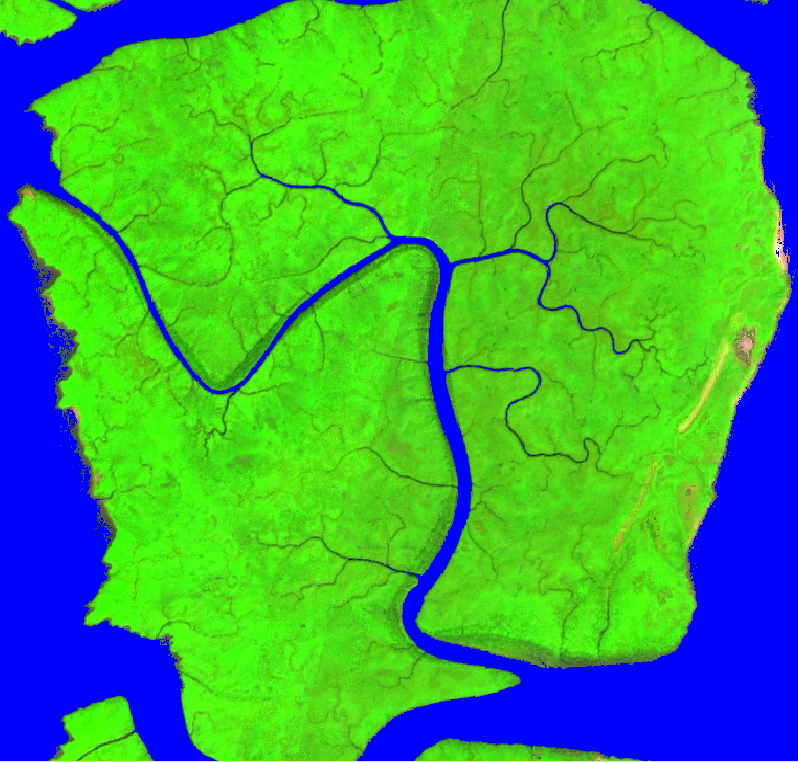
You’ll notice that new layers are loaded in the map, which include the edge detection and a water mask that identifies all marine and surface water (Fig. A3.2.1).

Question 2. Is the point well located to appropriately identify the water mask? What happens with turbid water?

Move the point around and see if it improves the automatic water masking. Turbid water can be an issue and may not be detected by the mask. Be certain that these muddy waters are not classified as mangrove later on.

Next, we create the land mask by inverting the water mask, and removing any areas with elevation greater than 40 m above sea level using the NASADEM (Digital Elevation Model from NASA) data collection. This will ensure we aren’t erroneously mapping mangroves far inland, where they don’t occur. You can of course change the elevation threshold according to your study area.

Next, we will buffer the area of interest to map mangroves only in areas where they might realistically be found. For this we will use the Global Mangrove Dataset from 2000 available in Earth Engine (note: this is one of several mangrove datasets; you could also have used other datasets such as Global Mangrove Watch or any other available raster data.)

The Global Mangrove Dataset was derived from Landsat 2000 (Giri et al. 2011); we will buffer 1000 m around it. The 1000 m buffer allows for the possibility that some mangroves were missed in the original map, and that mangroves might have expanded in some areas since 2000. You can change the buffer distance to any value suitable for your study area.

Question 3. Can the buffer distance or elevation threshold be changed to capture more mangroves or remove extra areas where mangroves aren’t likely to be found - and that we don’t need to classify? We don’t want to miss any mangrove areas, but we also want an efficient code that does not process areas that can’t be mangroves, which can add processing complexity and commit easily avoidable errors. To restrict the processing to the potential mangrove area, can you change the buffer distance or elevation threshold to best capture the area you are interested in?

We will now mask the mangrove buffer, create the area to classify and mask it from the data stack.

Code Checkpoint A32b. The book’s repository contains a script that shows what your code should look like at this point.

Section 3. Creating Training Data and Running and Evaluating a Random Forest  Classification

We will now automatically select mangrove and non-mangrove areas as training data. We use morphological image processing (see Chap. F3.2) to select areas deep inside the reference mangrove dataset; these are areas we can be sure are mangroves, because mangrove forests tend to be lost or deforested at the edges rather than in the interior. Using the same theory, we select areas far away from mangroves as our non-forest areas. This approach allows us to use a relatively older dataset from 2000 for current data training. We will extract mangrove and non-mangrove from the reference data.

We then use erosion and dilation (as described in Chap. F3.2) to identify areas at the center of mangrove forests and far from outside edges. We put everything together in a training layer where mangroves=1, non-mangroves=2, and everything else=0.

Question 4. How do the kernel radius and iteration parameters identify or miss important core mangrove areas?

To obtain good training data, we want samples located throughout the area of interest. Sometimes, if the mangroves are in very small patches, if the radius is too large, or if there are too many iterations, we don’t end up with enough core forest to sample.

Change the parameters to see what works best for you. You may need to zoom in to see the core mangrove areas.  

The next step is the classification (see Chap. F2.1). We will collect random samples from the training areas to train and run the random forest classifier. We will conduct two classifications. One is for validation, to obtain the test accuracy and determine how consistent the training areas are between two random samples.

The training accuracy is over 99%, which is very good. According to the substitution matrix, only a few training points seem to be confused when they are randomly replaced.

In addition, we can estimate variable importance, or how much each band contributes to the final random forest model. These are always good metrics to observe, as you could remove the least important bands from the training image if you wanted to.

Question 5. What are the most important bands in the classification model?

Question 6. Based on the chart, is one of the sensors more important in the classification model? Which bands? Why do you think that is?

Next, we will visualize the final classification. We can apply a filter to remove individual pixels, which effectively applies a minimum mapping unit (MMU). In this case, any areas with fewer than 25 connected pixels are filtered out.

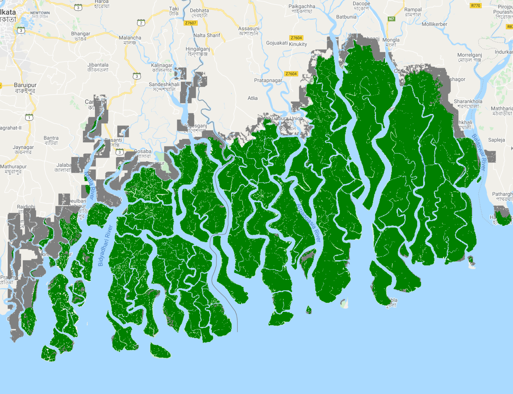
Your map window should resemble Fig. A3.2.2 with mangroves in green, and non-mangroves in gray.

Code Checkpoint A32c. The book’s repository contains a script that shows what your code should look like at this point.

In the Console window, you’ll see the substitution matrix, training accuracy, and a chart of variable importance.

Question 7. Do you notice any errors in the map? Omissions or commissions? How does the map compare to 2000?

Question 8. You should be able to see small differences in the mangrove extent since 2000. What do you see? What could be the causes for the changes?

Question 9.  How does the MMU parameter change the output map?

Try out different values and see what the results look like.

Synthesis

Assignment 1. With what you learned in this chapter, you can fuse Sentinel-1 and -2 data to create your own map of mangroves for anywhere in the world. You might now test out the approach in another part of the world, or use your own training data for a more refined classification model. You can add your own point data in the map and merge with the training data to improve a classification, or clean areas that need to be removed by drawing polygons and masking them in the classification.

Assignment 2. You can also add more indices, remove ones that aren’t as informative, create a map using earlier imagery, use the later date classification as reference data, and look for differences via post-classification change. Additional indices can be found in script A32s1 - Supplemental in the book's repository. Using these other indices, does that change your estimation of what areas are stable mangrove, and where have we observed gains or losses?

Conclusion

Mangroves are dynamic ecosystems that can expand over time, and that also can be lost through natural and anthropogenic causes. The power of Earth Engine lies in the cloud-based, lightning-fast, automated approach to workflows, particularly with automated training data collection. This process would take days when performed offline in traditional remote sensing software, especially over large areas. The Earth Engine approach is not only fast but also consistent. The same method can be applied to images from different dates to assess mangrove changes over time—both gain and loss.

Feedback

To review this chapter and make suggestions or note any problems, please go now to bit.ly/EEFA-review. You can find summary statistics from past reviews at bit.ly/EEFA-reviews-stats.

References

Cloud-Based Remote Sensing with Google Earth Engine. (n.d.). CLOUD-BASED REMOTE SENSING WITH GOOGLE EARTH ENGINE. https://www.eefabook.org/

Cloud-Based Remote Sensing with Google Earth Engine. (2024). In Springer eBooks. https://doi.org/10.1007/978-3-031-26588-4

Donchyts G, Schellekens J, Winsemius H, et al (2016) A 30 m resolution surface water mask including estimation of positional and thematic differences using Landsat 8, SRTM and OpenStreetMap: A case study in the Murray-Darling basin, Australia. Remote Sens 8:386. https://doi.org/10.3390/rs8050386

Esch T, Üreyen S, Zeidler J, et al (2018) Exploiting big Earth data from space–first experiences with the TimeScan processing chain. Big Earth Data 2:36–55. https://doi.org/10.1080/20964471.2018.1433790

Giri C, Ochieng E, Tieszen LL, et al (2011) Status and distribution of mangrove forests of the world using Earth observation satellite data. Glob Ecol Biogeogr 20:154–159. https://doi.org/10.1111/j.1466-8238.2010.00584.x

Mullissa A, Vollrath A, Odongo-Braun C, et al (2021) Sentinel-1 SAR backscatter analysis ready data preparation in Google Earth Engine. Remote Sens 13:1954. https://doi.org/10.3390/rs13101954

Vollrath A, Mullissa A, Reiche J (2020) Angular-based radiometric slope correction for Sentinel-1 on Google Earth Engine. Remote Sens 12:1867. https://doi.org/10.3390/rs12111867

Wang D, Wan B, Qiu P, et al (2018) Evaluating the performance of Sentinel-2, Landsat 8 and Pléiades-1 in mapping mangrove extent and species. Remote Sens 10:1468. https://doi.org/10.3390/rs10091468

Yancho JMM, Jones TG, Gandhi SR, et al (2020) The Google Earth Engine mangrove mapping methodology (GEEMMM). Remote Sens 12:1–35. https://doi.org/10.3390/rs12223758