Cloud-Based Remote Sensing with Google Earth Engine

Fundamentals and Applications

Part F5: Vectors and Tables

In addition to raster data processing, Earth Engine supports a rich set of vector processing tools. This Part introduces you to the vector framework in Earth Engine, shows you how to create and to import your vector data, and how to combine vector and raster data for analyses.

Chapter F5.0: Exploring Vectors

Authors

AJ Purdy, Ellen Brock, David Saah

Overview

In this chapter, you will learn about features and feature collections and how to use them in conjunction with images and image collections in Earth Engine. Maps are useful for understanding spatial patterns, but scientists often need to extract statistics to answer a question. For example, you may make a false-color composite showing which areas of San Francisco are more “green”—i.e., have more healthy vegetation—than others, but you will likely not be able to directly determine which block in a neighborhood is the most green. This tutorial will demonstrate how to do just that by utilizing vectors.

As described in Chap. F4.0, an important way to summarize and simplify data in Earth Engine is through the use of reducers. Reducers operating across space were used in Chap. F3.0, for example, to enable image regression between bands. More generally, chapters in Part F3 and Part F4 used reducers mostly to summarize the values across bands or images on a pixel-by-pixel basis. What if you wanted to summarize information within the confines of given spatial elements- for example, within a set of polygons? In this chapter, we will illustrate and explore Earth Engine’s method for doing that, which is through a reduceRegions call.

Learning Outcomes

• Uploading and working with a shapefile as an asset to use in Earth Engine.
• Creating a new feature using the geometry tools.
• Importing and filtering a feature collection in Earth Engine.
• Using a feature to clip and reduce image values within a geometry.
• Use reduceRegions to summarize an image in irregular neighborhoods.
• Exporting calculated data to tables with Tasks.

Assumes you know how to:

• Import images and image collections, filter, and visualize (Part F1).
• Calculate and interpret vegetation indices (Chap. F2.0).
• Use drawing tools to create points, lines, and polygons (Chap. F2.1).

Github Code link for all tutorials

This code base is collection of codes that are freely available from different authors for google earth engine.

Github Source

Introduction to Theory 

In the world of geographic information systems (GIS), data is typically thought of in one of two basic data structures: raster and vector. In previous chapters, we have principally been focused on raster data—data using the remote sensing vocabulary of pixels, spatial resolution, images, and image collections. Working within the vector framework is also a crucial skill to master. If you don’t know much about GIS, you can find any number of online explainers of the distinctions between these data types, their strengths and limitations, and analyses using both data types. Being able to move fluidly between a raster conception and a vector conception of the world is powerful, and is facilitated with specialized functions and approaches in Earth Engine.    

For our purposes, you can think of vector data as information represented as points (e.g., locations of sample sites), lines (e.g., railroad tracks), or polygons (e.g., the boundary of a national park or a neighborhood). Line data and polygon data are built up from points: for example, the latitude and longitude of the sample sites, the points along the curve of the railroad tracks, and the corners of the park that form its boundary. These points each have a highly specific location on Earth’s surface, and the vector data formed from them can be used for calculations with respect to other layers. As will be seen in this chapter, for example, a polygon can be used to identify which pixels in an image are contained within its borders. Point-based data have already been used in earlier chapters for filtering image collections by location (see Part F1), and can also be used to extract values from an image at a point or a set of points (see Chap. F5.2). Lines possess the dimension of length and have similar capabilities for filtering image collections and accessing their values along a transect. In addition to using polygons to summarize values within a boundary, they can be used for other, similar purposes—for example, to clip an image.

As you have seen, raster features in Earth Engine are stored as an Image or as part of an ImageCollection. Using a similar conceptual model, vector data in Earth Engine is stored as a Feature or as part of a FeatureCollection. Features and feature collections provide useful data to filter images and image collections by their location, clip images to a boundary, or statistically summarize the pixel values within a region.

In the following example, you will use features and feature collections to identify which city block near the University of San Francisco (USF) campus is the most green.

Practicum

Section 1. Using Geometry Tools to Create Features in Earth Engine

To demonstrate how geometry tools in Earth Engine work, let’s start by creating a point, and two polygons to represent different elements on the USF campus.

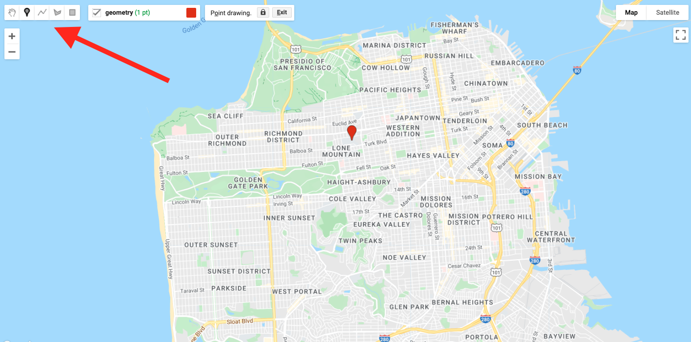
Click on the geometry tools in the top left of the Map pane and create a point feature. Place a new point where USF is located (see Fig. F5.0.1).

Use Google Maps to search for “Harney Science Center” or “Lo Schiavo Center for Science.” Hover your mouse over the Geometry Imports to find the +new layer menu item and add a new layer to delineate the boundary of a building on campus.

Next, create another new layer to represent the entire campus as a polygon.

After you create these layers, rename the geometry imports at the top of your script. Name the layers usf_point, usf_building, and usf_campus. These names are used within the script shown in Fig. F5.0.2.

Code Checkpoint F50a. The book’s repository contains a script that shows what your code should look like at this point. 

Section 2. Loading Existing Features and Feature Collections in Earth Engine

If you wish to have the exact same geometry imports in this chapter for the rest of this exercise, begin this section using the code at the Code Checkpoint above.

Next, you will load a city block dataset to determine the amount of vegetation on blocks near USF. The code below imports an existing feature dataset in Earth Engine. The Topologically Integrated Geographic Encoding and Referencing (TIGER) boundaries are census-designated boundaries that are a useful resource when comparing socioeconomic and diversity metrics with environmental datasets in the United States.

You should now have the geometry for USF’s campus and a layer added to your map that is not visualized for census blocks across the United States. Next, we will use neighborhood data to spatially filter the TIGER feature collection for blocks near USF’s campus.

Section 3. Importing Features into Earth Engine

There are many image collections loaded in Earth Engine, and they can cover a very large area that you might want to study. Borders can be quite intricate (for example, a detailed coastline), and fortunately there is no need for you to digitize the intricate boundary of a large geographic area. Instead, we will show how to find a spatial dataset online, download the data, and load this into Earth Engine as an asset for use.

Find a Spatial Dataset of San Francisco Neighborhoods

Use your internet searching skills to locate the “Analysis Neighborhoods” dataset covering San Francisco. This data might be located in a number of places, including DataSF, the City of San Francisco’s public-facing data repository.

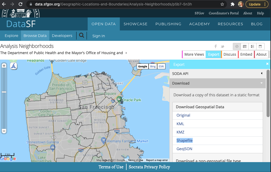
After you find the Analysis Neighborhoods layer, click Export and select Shapefile (Fig. F5.0.3). Keep track of where you save the zipped file, as we will load this into Earth Engine. Shapefiles contain vector-based data—points, lines, polygons—and include a number of files, such as the location information, attribute information, and others.

Extract the folder to your computer. When you open the folder, you will see that there are actually many files. The extensions (.shp, .dbf, .shx, .prj) all provide a different piece of information to display vector-based data. The .shp file provides data on the geometry. The .dbf file provides data about the attributes. The .shx file is an index file. Lastly, the .prj file describes the map projection of the coordinate information for the shapefile. You will need to load all four files to create a new feature asset in Earth Engine.

Upload SF Neighborhoods File as an Asset

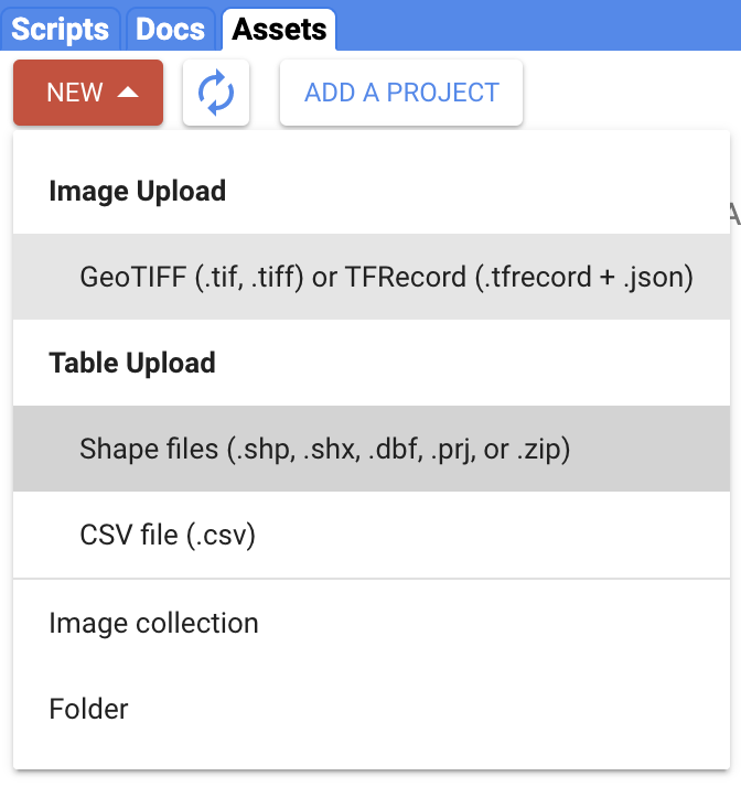
Navigate to the Assets tab (near Scripts). Select New > Table Upload > Shape files (Fig. F5.0.4).

Select Files and Name Asset

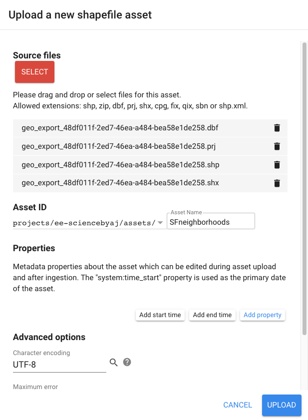
Click the Select button and then use the file navigator to select the component files of the shapefile structure (i.e., .shp, .dbf, .shx, and .prj) (Fig. F5.0.5). Assign an Asset Name so you can recognize this asset.

Uploading the asset may take a few minutes. The status of the upload is presented under the Tasks tab. After your asset has been successfully loaded, click on the asset in the Assets folder and find the collection ID. Copy this text and use it to import the file into your Earth Engine analysis.

Assign the asset to the table (collection) ID using the script below. Note that you will need to replace 'path/to/your/asset/assetname' with the actual path copied in the previous step.

Note that if you have any trouble with loading the FeatureCollection using the technique above, you can follow directions in the Checkpoint script below to use an existing asset loaded for this exercise.

Code Checkpoint F50b. The book’s repository contains a script that shows what your code should look like at this point.

Section 4. Filtering Feature Collections by Attributes

Filter by Geometry of Another Feature

First, let’s find the neighborhood associated with USF. Use the first point you created to find the neighborhood that intersects this point; filterBounds is the tool that does that, returning a filtered feature.

Now, filter the blocks layer by USF’s neighborhood and visualize it on the map.

Filter by Feature (Attribute) Properties

In addition to filtering a FeatureCollection by the location of another feature, you can also filter it by its properties. First, let’s print the usfTiger variable to the Console and inspect the object.

You can click on the feature collection name in the Console to uncover more information about the dataset. Click on the columns to learn about what attribute information is contained in this dataset. You will notice this feature collection contains information on both housing ('housing10') and population ('pop10').

Now you will filter for blocks with just the right amount of housing units. You don’t want it too dense, nor do you want too few neighbors.

Filter the blocks to have fewer than 250 housing units.

Now filter the already-filtered blocks to have more than 50 housing units.

Now, let’s visualize what this looks like.

We have combined spatial and attribute information to narrow the set to only those blocks that meet our criteria of having between 50 and 250 housing units.

Print Feature (Attribute) Properties to Console

We can print out attribute information about these features. The block of code below prints out the area of the resultant geometry in square meters.

The next block of code reduces attribute information and prints out the mean of the housing10 column.

Both of the above sections of code provide meaningful information about each feature, but they do not tell us which block is the most green. The next section will address that question.

Code Checkpoint F50c. The book’s repository contains a script that shows what your code should look like at this point. 

Section 5. Reducing Images Using Feature Geometry

Now that we have identified the blocks around USF’s campus that have the right housing density, let’s find which blocks are the greenest.

The Normalized Difference Vegetation Index (NDVI), presented in detail in Chap. F2.0, is often used to compare the greenness of pixels in different locations. Values on land range from 0 to 1, with values closer to 1 representing healthier and greener vegetation than values near 0.

Create an NDVI Image

The code below imports the Landsat 8 ImageCollection as landsat8. Then, the code filters for images in 2021. Lastly, the code sorts the images from 2021 to find the least cloudy day.

The next section of code assigns the near-infrared band (B5) to variable nir and assigns the red band (B4) to red. Then the bands are combined together to compute NDVI as (nir − red)/(nir + red).

Clip the NDVI Image to the Blocks Near USF

Next, you will clip the NDVI layer to only show NDVI over USF’s neighborhood.

The first section of code provides visualization settings.

The second block of code clips the image to our filtered housing layer.

The NDVI map for all of San Francisco is interesting, and shows variability across the region. Now, let’s compute mean NDVI values for each block of the city.

Compute NDVI Statistics by Block

The code below uses the clipped image ndviUSFblocks and computes the mean NDVI value within each boundary. The scale provides a spatial resolution for the mean values to be computed on.

Now we’ll use Earth Engine to find out which block is greenest.  

Export Table of NDVI Data by Block from Earth Engine to Google Drive

Just as we loaded a feature into Earth Engine, we can export information from Earth Engine. Here, we will export the NDVI data, summarized by block, from Earth Engine to a Google Drive space so that we can interpret it in a program like Google Sheets or Excel.

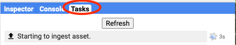
When you run this code, you will notice that you have the Tasks tab highlighted on the top right of the Earth Engine Code Editor (Fig. F5.0.6). You will be prompted to name the directory when exporting the data.

After you run the task, the file will be saved to your Google Drive. You have now brought a feature into Earth Engine and also exported data from Earth Engine.

Code Checkpoint F50d. The book’s repository contains a script that shows what your code should look like at this point. 

Section 6. Identifying the Block in the Neighborhood Surrounding USF with the Highest NDVI

You are already familiar with filtering datasets by their attributes. Now you will sort a table and select the first element of the table.

If you expand the feature of ndviPerBlockSortedFirst in the Console, you will be able to identify the blockid10 value of the greenest block and the mean NDVI value for that area.

Another way to look at the data is by exporting the data to a table. Open the table using Google Sheets or Excel. You should see a column titled “mean.” Sort the mean column in descending order from highest NDVI to lowest NDVI, then use the blockid10 attribute to filter our feature collection one last time and display the greenest block near USF.

Code Checkpoint F50e. The book’s repository contains a script that shows what your code should look like at this point. 

Synthesis

Now it’s your turn to use both feature classes and to reduce data using a geographic boundary. Create a new script for an area of interest and accomplish the following assignments.

Assignment 1. Create a study area map zoomed to a certain feature class that you made.

Assignment 2. Filter one feature collection using feature properties.

Assignment 3. Filter one feature collection based on another feature’s location in space.

Assignment 4. Reduce one image to the geometry of a feature in some capacity; e.g., extract a mean value or a value at a point.

Conclusion

In this chapter, you learned how to import features into Earth Engine. In Sect. 1, you created new features using the geometry tools and loaded a feature from Earth Engine’s Data Catalog. In Sect. 2, you loaded a shapefile to an Earth Engine asset. In Sect. 3, you filtered feature collections based on their properties and locations. Finally, in Sects. 4 and 5, you used a feature collection to reduce an image, then exported the data from Earth Engine. Now you have all the tools you need to load, filter, and apply features to extract meaningful information from images using vector features in Earth Engine.

Feedback

To review this chapter and make suggestions or note any problems, please go now to bit.ly/EEFA-review. You can find summary statistics from past reviews at bit.ly/EEFA-reviews-stats.

References

Cloud-Based Remote Sensing with Google Earth Engine. (n.d.). CLOUD-BASED REMOTE SENSING WITH GOOGLE EARTH ENGINE. https://www.eefabook.org/

Cloud-Based Remote Sensing with Google Earth Engine. (2024). In Springer eBooks. https://doi.org/10.1007/978-3-031-26588-4