Cloud-Based Remote Sensing with Google Earth Engine

Fundamentals and Applications

Part F4: Interpreting Image Series

One of the paradigm-changing features of Earth Engine is the ability to access decades of imagery without the previous limitation of needing to download all the data to a local disk for processing. Because remote-sensing data files can be enormous, this used to limit many projects to viewing two or three images from different periods. With Earth Engine, users can access tens or hundreds of thousands of images to understand the status of places across decades.

Chapter F4.9: Exploring Lagged Effects in Time Series 

Authors

Andréa Puzzi Nicolau, Karen Dyson, David Saah, Nicholas Clinton

Overview

In this chapter, we will introduce lagged effects to build on previous work in modeling time-series data. Time-lagged effects occur when an event at one point in time impacts dependent variables at a later point in time. You will be introduced to concepts of autocovariance and autocorrelation, cross-covariance and cross-correlation, and auto-regressive models. At the end of this chapter, you will be able to examine how variables relate to one another across time, and to fit time series models that take into account lagged events. 

Learning Outcomes

• Using the ee.Join function to create time-lagged collections.
• Calculating autocovariance and autocorrelation.
• Calculating cross-covariance and cross-correlation.
• Fitting auto-regressive models.

Assumes you know how to:

• Import images and image collections, filter, and visualize (Part F1).
• Perform basic image analysis: select bands, compute indices, create masks, classify images (Part F2).
• ​​Create a graph using ui.Chart (Chap. F1.3).
• Write a function and map it over an ImageCollection (Chap. F4.0).
• Mask cloud, cloud shadow, snow/ice, and other undesired pixels (Chap. F4.3).
• Fit linear and nonlinear functions with regression in an ImageCollection time series (Chap. F4.6).

Github Code link for all tutorials

This code base is collection of codes that are freely available from different authors for google earth engine.

Github Source

Introduction to Theory

While fitting functions to time series allows you to account for seasonality in your models, sometimes the impact of a seasonal event does not impact your dependent variable until the next month, the next year, or even multiple years later. For example, coconuts take 18–24 months to develop from flower to harvestable size. Heavy rains during the flower development stage can severely reduce the number of coconuts that can be harvested months later, with significant negative economic repercussions. These patterns—where events in one time period impact our variable of interest in later time periods—are important to be able to include in our models.

In this chapter, we introduce lagged effects into our previous discussions on interpreting time-series data (Chaps. F4.6 and F4.7). Being able to integrate lagged effects into our time-series models allows us to address many important questions. For example, streamflow can be accurately modeled by taking into account previous streamflow, rainfall, and soil moisture; this improved understanding helps predict and mitigate the impacts of drought and flood events made more likely by climate change (Sazib et al. 2020). As another example, time-series lag analysis was able to determine that decreased rainfall was associated with increases in livestock disease outbreaks one year later in India (Karthikeyan et al. 2021).

Practicum

Section 1. Autocovariance and Autocorrelation

Before we dive into autocovariance and autocorrelation, let’s set up an area of interest and dataset that we can use to illustrate these concepts. We will work with a detrended time series (as seen in Chap. F4.6) based on the USGS Landsat 8 Level 2, Collection 2, Tier 1 image collection. Copy and paste the code below to filter the Landsat 8 collection to a point of interest over California and specific dates, and apply the pre-processing function—to mask clouds (as seen in Chap. F4.3) and to scale and add variables of interest (as seen in Chap. F4.6).

Next, copy and paste the code below to estimate the linear trend using the linearRegression reducer, and remove that linear trend from the time series.

Now let’s turn to autocovariance and autocorrelation. The autocovariance of a time series refers to the dependence of values in the time series at time t with values at time h =t − lag. The autocorrelation is the correlation between elements of a dataset at one time and elements of the same dataset at a different time. The autocorrelation is the autocovariance normalized by the standard deviations of the covariates. Specifically, we assume our time series is stationary, and define the autocovariance and autocorrelation following Shumway and Stoffer (2019). Comparing values at time t to previous values is useful not only for computing autocovariance, but also for a variety of other time series analyses as you'll see shortly.

To combine image data with previous values in Earth Engine, the first step is to join the previous values to the current values. To do that, we will use a ee.Join function to create what we'll call a lagged collection. Copy and paste the code below to define a function that creates a lagged collection.

This function joins a collection to itself, using a filter that gets all the images before each image’s date that are within a specified time difference (in days) of each image. That list of previous images within the lag time is stored in a property of the image called images, sorted reverse chronologically. For example, to create a lagged collection from the detrended Landsat imagery, copy and paste:

Why 17 days? Recall that the temporal cadence of Landsat is 16 days. Specifying 17 days in the join gets one previous image, but no more.

Now, we will compute the autocovariance using a reducer that expects a set of one-dimensional arrays as input. So pixel values corresponding to time t need to be stacked with pixel values at time t − lag as multiple bands in the same image. Copy and paste the code below to define a function to do so, and apply it to merge the bands from the lagged collection.

Now the bands from time t and h are all in the same image. Note that the band name of a pixel at time h, ph, was the same as time t, pt (band name is “NDVI” in this case). During the merging process, it gets a '_1' appended to it (e.g. NDVI_1).

You can print the image collection to check the band names of one of the images. Copy and paste the code below to map a function to convert the merged bands to arrays with bands pt and ph, and then reduce it with the covariance reducer. We use a parallelScale factor of 8 in the reduce function to avoid the computation to run out of memory (this is not always needed). Note that the output of the covariance reducer is an array image, in which each pixel stores a 2x2 variance-covariance array. The off-diagonal elements are covariance, which you can map directly using the arrayGet function.

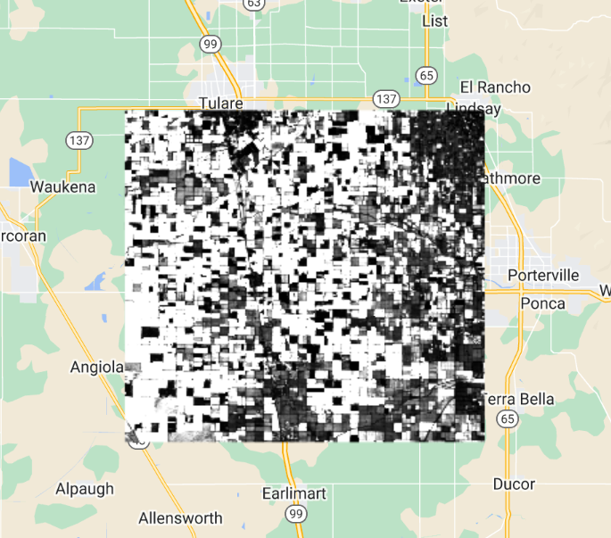
Inspect the pixel values of the resulting covariance image (Fig. F4.9.1). The covariance is positive when the greater values of one variable (at time t) mainly correspond to the greater values of the other variable (at time h), and the same holds for the lesser values, therefore, the values tend to show similar behavior. In the opposite case, when the greater values of a variable correspond to the lesser values of the other variable, the covariance is negative.

The diagonal elements of the variance-covariance array are variances. Copy and paste the code below to define and map a function to compute correlation (Fig. F4.9.2) from the variance-covariance array.

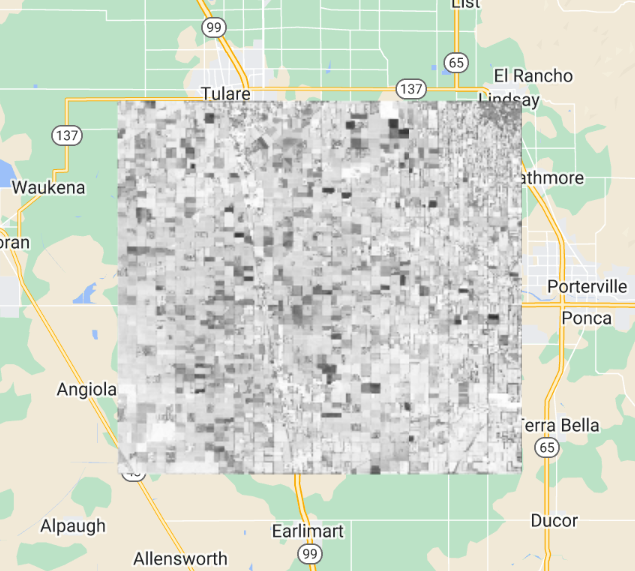
Higher positive values indicate higher correlation between the elements of the dataset, and lower negative values indicate the opposite.

It's worth noting that you can do this for longer lags as well. Of course, that images list will fill up with all the images that are within lag of t. Those other images are also useful—for example, in fitting autoregressive models as described later.

Code Checkpoint F49a. The book’s repository contains a script that shows what your code should look like at this point.

Section 2. Cross-Covariance and Cross-Correlation

Cross-covariance is analogous to autocovariance, except instead of measuring the correspondence between a variable and itself at a lag, it measures the correspondence between a variable and a covariate at a lag. Specifically, we will define the cross-covariance and cross-correlation according to Shumway and Stoffer (2019). 

You already have all the code needed to compute cross-covariance and cross-correlation. But you do need a time series of another variable. Suppose we postulate that NDVI is related in some way to the precipitation before the NDVI was observed. To estimate the strength of this relationship in every pixel, copy and paste the code below to the existing script to load precipitation, join, merge, and reduce as previously:

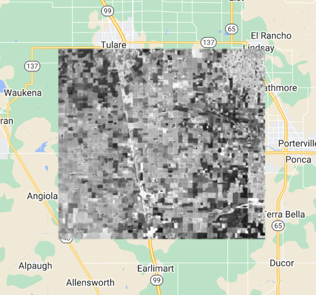
What do you observe from this result? Looking at the cross-correlation image (Fig. F4.9.3), do you observe high values where you would expect high NDVI values (vegetated areas)? One possible drawback of this computation is that it's only based on five days of precipitation, whichever five days came right before the NDVI image.

Perhaps precipitation in the month before the observed NDVI is relevant? Copy and paste the code below to test the 30-day lag idea.

Observe that the only change is to the merge method. Instead of merging the bands of the NDVI image and the covariate (precipitation), the entire list of precipitation is summed and added as a band (eliminating the need for iterate).

Which changes do you notice between the cross-correlation images—5 days lag vs. 30 days lag (Fig. F4.9.4)?. You can use the Inspector tool to assess if the correlation increased or not at vegetated areas.

As long as there is sufficient temporal overlap between the time series, these techniques could be extended to longer lags and longer time series.

Code Checkpoint F49b. The book’s repository contains a script that shows what your code should look like at this point.

Section 3. Auto-Regressive Models

The discussion of autocovariance preceded this section in order to introduce the concept of lag. Now that you have a way to get previous values of a variable, it's worth considering auto-regressive models. Suppose that pixel values at time t depend in some way on previous pixel values—auto-regressive models are time series models that use observations from previous time steps as input to a regression equation to predict the value at the next time step. If you have observed significant, non-zero autocorrelations in a time series, this is a good assumption. Specifically, you may postulate a linear model such as the following, where pt is a pixel at time t, and et is a random error (Chap. F4.6):

pt =β0 + β1pt-1 + β2pt-2 + et                                        (F4.9.1)

To fit this model, you need a lagged collection as created previously, except with a longer lag (e.g., lag =34 days). The next steps are to merge the bands, then reduce with the linear regression reducer.

Copy and paste the line below to the existing script to create a lagged collection, where the images list stores the two previous images:

Copy and paste the code below to merge the bands of the lagged collection such that each image has bands at time t and bands at times t - 1,..., t − lag. Note that it's necessary to filter out any images that don't have two previous temporal neighbors.

Now, copy and paste the code below to fit the regression model using the linearRegression reducer.

We can compute the fitted values using the expression function in Earth Engine. Because this model is a function of previous pixel values, which may be masked, if any of the inputs to equation F4.9.1 are masked, the output of the equation will also be masked. That's why you should use an expression here, unlike the previous linear models of time. Copy and paste the code below to compute the fitted values.

Finally, copy and paste the code below to plot the results (Fig. F4.9.5). We will use a specific point defined as pt. Note the missing values that result from masked data. If you run into computation errors, try commenting the Map.addLayer calls from previous sections to save memory.

At this stage, note that the missing data has become a real problem. Any data point for which at least one of the previous points is masked or missing is also masked.

Code Checkpoint F49c. The book’s repository contains a script that shows what your code should look like at this point.

It may be possible to avoid this problem by substituting the output from equation F4.9.1 (the modeled value) for the missing or masked data. Unfortunately, the code to make that happen is not straightforward. You can check a solution in the following Code Checkpoint:

Code Checkpoint F49d. The book’s repository contains a script that shows what your code should look like at this point.

Synthesis

Assignment 1. Analyze cross-correlation between NDVI and soil moisture, or precipitation and soil moisture, for example. Earth Engine contains different soil moisture datasets in its catalog (e.g., NASA-USDA SMAP, NASA-GLDAS). Try increasing the lagged time and see if it makes any difference. Alternatively, you can pick any other environmental variable/index (e.g., a different vegetation index: EVI instead of NDVI, for example) and analyze its autocorrelation.

Conclusion

In this chapter, we learned how to use autocovariance and autocorrelation to explore the relationship between elements of a time series at multiple time steps. We also explored how to use cross-covariance and cross-correlation to examine the relationship between elements of two time series at different points in time. Finally, we used auto-regressive models to regress the elements of a time series with elements of the same time series at a different point in time. With these skills, you can now examine how events in one time period impact your variable of interest in later time periods. While we have introduced the linear approach to lagged effects, these ideas can be expanded to more complex models.

Feedback

To review this chapter and make suggestions or note any problems, please go now to bit.ly/EEFA-review. You can find summary statistics from past reviews at bit.ly/EEFA-reviews-stats.

References

Cloud-Based Remote Sensing with Google Earth Engine. (n.d.). CLOUD-BASED REMOTE SENSING WITH GOOGLE EARTH ENGINE. https://www.eefabook.org/

Cloud-Based Remote Sensing with Google Earth Engine. (2024). In Springer eBooks. https://doi.org/10.1007/978-3-031-26588-4

Karthikeyan R, Rupner RN, Koti SR, et al (2021) Spatio-temporal and time series analysis of bluetongue outbreaks with environmental factors extracted from Google Earth Engine (GEE) in Andhra Pradesh, India. Transbound Emerg Dis 68:3631–3642. https://doi.org/10.1111/tbed.13972

Sazib N, Bolten J, Mladenova I (2020) Exploring spatiotemporal relations between soil moisture, precipitation, and streamflow for a large set of watersheds using Google Earth Engine. Water (Switzerland) 12:1371. https://doi.org/10.3390/w12051371

Shumway RH, Stoffer DS (2019) Time Series: A Data Analysis Approach Using R. Chapman and Hall/CRC