Cloud-Based Remote Sensing with Google Earth Engine

Fundamentals and Applications

Part F5: Vectors and Tables

In addition to raster data processing, Earth Engine supports a rich set of vector processing tools. This Part introduces you to the vector framework in Earth Engine, shows you how to create and to import your vector data, and how to combine vector and raster data for analyses.

Chapter F5.4: GEEDiT - Digitizing From Satellite Imagery

Author

James Lea

Overview 

Earth surface margins and features are often of key interest to environmental scientists. A coastline, the terminus of a glacier, the outline of a landform, and many other examples can help illustrate past, present, and potential future environmental change. The information gained from these features can be used to achieve greater understanding of the underlying processes that are controlling these systems, to monitor their responses to ongoing environmental changes, and to assess and inform wider socio-economic impacts at local to global scales.

While it is common practice in remote sensing to automate identification of margins from imagery, these attempts are not always successful or transferable between seasons or locations. Furthermore, in some circumstances the nature of the margins that need to be identified means that implementing automated approaches are not always necessary, desirable, or even possible. In such cases, user-led manual digitization of margins may be the only appropriate way to generate accurate, user-verified data. However, users who wish to undertake this analysis at scale often face the time-consuming challenge of having to download and process large volumes of satellite imagery. Furthermore, issues such as internet connection speed, local storage capacity, and computational processing power availability can potentially limit or even preclude this style of analysis, leading to a fundamental inequality in the ability of users to generate datasets of comparable standards.

The Google Earth Engine Digitisation Tool (GEEDiT) is built to allow any researcher to rapidly access satellite imagery and directly digitize margins as lines or polygons. With a simple user interface and no need to download enormous images, GEEDiT leverages Earth Engine’s cloud computing power and its access to satellite image repositories (Lea, 2018). When the delineated vector margins are exported, they are also appended with standardized metadata from the source imagery. In doing so, users can easily trace back to which images associate with which digitized margins, facilitating reproducibility, independent verification, and building of easily shareable and transferable datasets (e.g. Goliber et al. 2022). Since GEEDiT is used through a graphical user interface, it requires no coding ability in Earth Engine to use it.

GEEDiT has been used for research in glaciology (e.g., Tuckett et al. 2019; Fahrner et al. 2021), hydrology (e.g., Boothroyd et al. 2021; Scheingross et al. 2021) and lake extent (e.g., Kochtitzky et al. 2020; Field et al. 2021) in addition to other fields. Version 2 of GEEDiT was released in early 2022 with improved functionality, usability, and access to new datasets.

Learning Outcomes

• Understanding how to use the GEEDiT v2 interface and export data from it.
• Becoming aware of some of the new functionality introduced in GEEDiT v2.
• Learning about potential options to customize GEEDiT v2 visualization parameters.

Assumes you know how to:

• Use drawing tools to create points, lines, and polygons (Chap. F2.1).
• Recognize similarities and differences among satellite spectral bands (Part F1, Part F2, Part F3).

Github Code link for all tutorials

This code base is collection of codes that are freely available from different authors for google earth engine.

Github Source

Introduction to Theory

As a tool, GEEDiT came about due to the author’s frustration with the requirement to download, process, and visualize significant volumes of satellite imagery for simple margin analysis, in addition to the tedious steps required for appending comprehensive and consistent metadata to them. GEEDiT was built to take advantage of Earth Engine’s capability for rapid cloud-based data access, processing and visualization, and potential for fully automated assignment of metadata.

GEEDiT allows users to visualize, review, and analyze an image in potentially a few seconds, whereas previously downloading and processing a single image would have taken considerably longer in a desktop GIS environment. Consequently, GEEDiT users can obtain margin data from significantly more imagery than was previously possible in the time available to them. Users can create larger, more spatially and temporally comprehensive datasets compared to traditional approaches, with automatically appended metadata also allowing easier dataset filtering, and tracing of data back to original source imagery. Where coding-based analysis of GEEDiT output is applied, the standardization of metadata also facilitates the transferability of code between datasets, and assists in the collation of homogenized margin and feature datasets that have been generated by multiple users (e.g. Goliber et al. 2022).

GEEDiT version 2 (hereafter GEEDiT) was released in January 2022 to provide improvements to the user experience of the tool, and the imagery data that it can access. Similar to version 1, it is a graphical user interface (GUI) built entirely within Earth Engine’s JavaScript API. This chapter provides a walkthrough of GEEDiT’s user interface, alongside information on how users can get the most out of its functionality.

Practicum

Code Checkpoint F54a. The book’s repository contains information about accessing the interface for GEEDiT.

Below, each step required to extract data from GEEDiT is described, using an example of digitizing the margin of a Greenlandic marine terminating glacier.

Section 1. Loading GEEDiT and Selecting Imagery Options and a Location

Click on the link to GEEDiT v2.02 Tier 1, to open the GUI in a new tab as shown in Fig. F5.4.1. If you are interested in the underlying code, you can view this in the Code Editor. Resize the view to maximize the map portion of the Earth Engine interface. If the interface does not appear, click the Run button above the Code Editor at the top of the page.

Section 1.1. Description of Starting Page Interface

Brief instructions on how to use the GUI are given at the bottom left of the interface, while image selection options are provided on the right (Fig. F5.4.2).

In this panel you can define the date range, month range, maximum allowable cloud cover, export task frequency, and satellite platforms for the images you want to analyze. Each of these are explained in turn below:

• Define start/end dates in YYYY-MM-DD format: These fields provide text boxes for you to define the date range of interest. The default start date is given as 1950-01-01, and the end date is the date the tool is being run. In this example we use the default settings, so you do not need to make any changes to the default values. However, common issues that arise using this functionality include:

• Not entering a date that is compatible with the YYYY-MM-DD format, including: placing days, months and years in the wrong order (e.g., 02-22-2022); and not using ‘-’ as a separator (e.g., 2022/22/02)
• Entering a date that cannot exist (e.g., 2022-09-31)
• Not including a leading 0 for single digit days or months (e.g., 2022-2-2)
• Not entering the full four-digit year (e.g., 22-02-02)
• Typographical errors

• Month start and month end: These are optional dropdown menus that allow users to obtain imagery only from given ranges of months within the previously defined date range. If users do not define these, imagery for the full year will be returned. In some cases (e.g., analysis of imagery during the austral summer) users may wish to obtain imagery from a month range that may span the year end (e.g., November to February). For this month range, this can be achieved by selecting a start month of 11, and a month end of 2. Given that glacier margins are often clearest and easiest to identify during the summer months, set the start month to July (7) and end month to September (9).
• Max. cloud cover: This field filters imagery by cloud cover metadata values that are appended to imagery obtained from optical satellite platforms, such as Landsat, Sentinel-2, and ASTER satellites. The names of the metadata that hold this information vary between these satellite platforms and are 'CLOUD_COVER', 'CLOUDY_PIXEL_PERCENTAGE' and 'CLOUDCOVER' respectively. Values associated with these image metadata represent automatically derived estimates of the percentage cloud cover of an entire image scene. These are calculated in different ways for the different satellites depending on the processing chain performed by NASA/ESA when the imagery was acquired.

Also, note that Sentinel-2 and ASTER imagery footprints are smaller than those of Landsat, meaning that 1% cloud cover for a Landsat image will cover a larger geographic area than 1% of a Sentinel-2 or ASTER image. Here we use the default setting (maximum 20% cloud cover), so you can leave this field unchanged.

• Automatically create data export task every n images: This will generate a data export task in Earth Engine for every n images viewed, where n is the value entered. The reason for including this as an option is that manual digitization features from imagery can be time-consuming depending on the level of detail required or number of features on an image. While rare, data losses can result from internet connection dropout, computer crashes, or the Earth Engine server going offline, so exporting digitized data frequently can help guard against this.
• Satellites: This menu provides a list of check boxes of all the satellite platforms from which imagery is available (Table F5.4.1). Descriptions of aspects of each satellite that users should be aware of when using these data for digitizing margins are described below.

Table F5.4.1 Key information for each satellite.

• ASTER L1T Radiance: The Advanced Spaceborne Thermal Emission and Reflection Radiometer (ASTER) collects both daytime and nighttime imagery (Some images may appear black.) The lack of a blue spectral band on ASTER means that it is not possible to visualize imagery as “true color” (i.e., red-green-blue), though it does allow imagery to be visualized at up to 15 m pixel resolution. The default color channel visualization for ASTER within GEEDiT is: B3N, near infrared in the red channel; B02, visible red in the green channel; B01, visible green/yellow in the blue channel .
• Landsat 4 Top of Atmosphere (TOA): The default image collection for Landsat 4 and all Landsat satellites listed below are taken from the TOA collections where the imagery has been calibrated for top of atmosphere reflectance (see Chander et al. 2009). The density of global coverage for Landsat 4 is variable, meaning that some regions may not possess any available images.
• Landsat 5 TOA:  Similar to Landsat 4, Landsat 5 has variable global coverage, meaning that some remote regions may have very few or no images.
• Landsat 7 Real-Time data, TOA reflectance: Beginning in 2003, a failure in the satellite’s scan-line corrector (SLC) mirror has resulted in data gaps on Landsat-7 imagery. The impact of this instrument failure is that stripes of missing data of increasing width emanate from near the center of the image scene, which can lead to challenges in continuous mapping of features or margins. The orbit of Landsat has also been drifting since 2017 meaning that the time of day when imagery is acquired for a given location has been getting earlier.
• Landsat 8 Real-Time data, TOA reflectance: Landsat 8 is automatically updated with new imagery as it becomes available. Note that the red, green, and blue bands are different for Landsat 8 compared to Landsat 4, 5, and 7 due to the addition of the coastal aerosol band as band 1.
• Sentinel-1 SAR GRD: Unlike other satellites that are listed as options in GEEDiT, Sentinel-1 is a synthetic aperture radar (SAR) satellite (i.e., it is an active source satellite operating in the radio frequency range, and does not collect visible spectrum imagery). A notable advantage of SAR imagery is that it is unaffected by cloud cover (cloud is transparent at radio frequencies) or sun illumination, providing full scene coverage for each image acquisition. Sentinel-1 transmits and receives reflected radio waves in either the vertical (V) or horizontal (H) polarizations, providing up to four bands available in Sentinel-1 data: VV, VH, HH and HV. In practice, a subset of these bands are usually acquired for each Sentinel-1 scene, with GEEDiT automatically visualizing the first available band. However, care needs to be taken when using this imagery for digitizing margins or features. This arises from the satellite being “side-looking,” which results in the location accuracy and ground resolution of imagery being variable, especially in areas of steep topography. The Sentinel-1 imagery available in Earth Engine is the ground range detected (GRD) product, meaning that a global digital elevation model (DEM) has been used to ortho-correct imagery. However, where there is a mismatch between the DEM used for ortho-correction and the true surface elevation (e.g., arising from glacier thinning), this may result in apparent shifts in topography between images that are non-negligible for analysis. This is especially the case where vectors are digitized from imagery obtained from both ascending and descending parts of its orbit. The magnitude of these apparent shifts will be dependent on the satellite look angle and mismatch between the DEM and true surface elevation, meaning that applying corrections without up-to-date DEMs is unfortunately non-trivial. For these reasons, it is suggested that where Sentinel-1 imagery is used to delineate margins or features that they are used for quantifying relative rather than absolute change, and significant care should be taken in the interpretation of margin and feature data generated from this imagery. As a result of these caveats, Sentinel-1 is not selected as a default option for visualization.
• Sentinel-2 MSI: Level 1C: The image collection included in GEEDiT is the Level 1C TOA data that provides global coverage. Also note that the ground control and ortho-correction for Sentinel-2 imagery is performed using a different DEM compared to Landsat satellites, meaning there may be small differences in geolocation consistency between imagery from these different platforms. Where margin or feature data from both these platform types are combined, users should therefore check the level of accuracy it is possible to derive, especially where fine scale differences between margins or features (e.g., a few pixels) are important (e.g., Brough et al. 2019).

Section 1.2. Visualizing Imagery at a Given Location

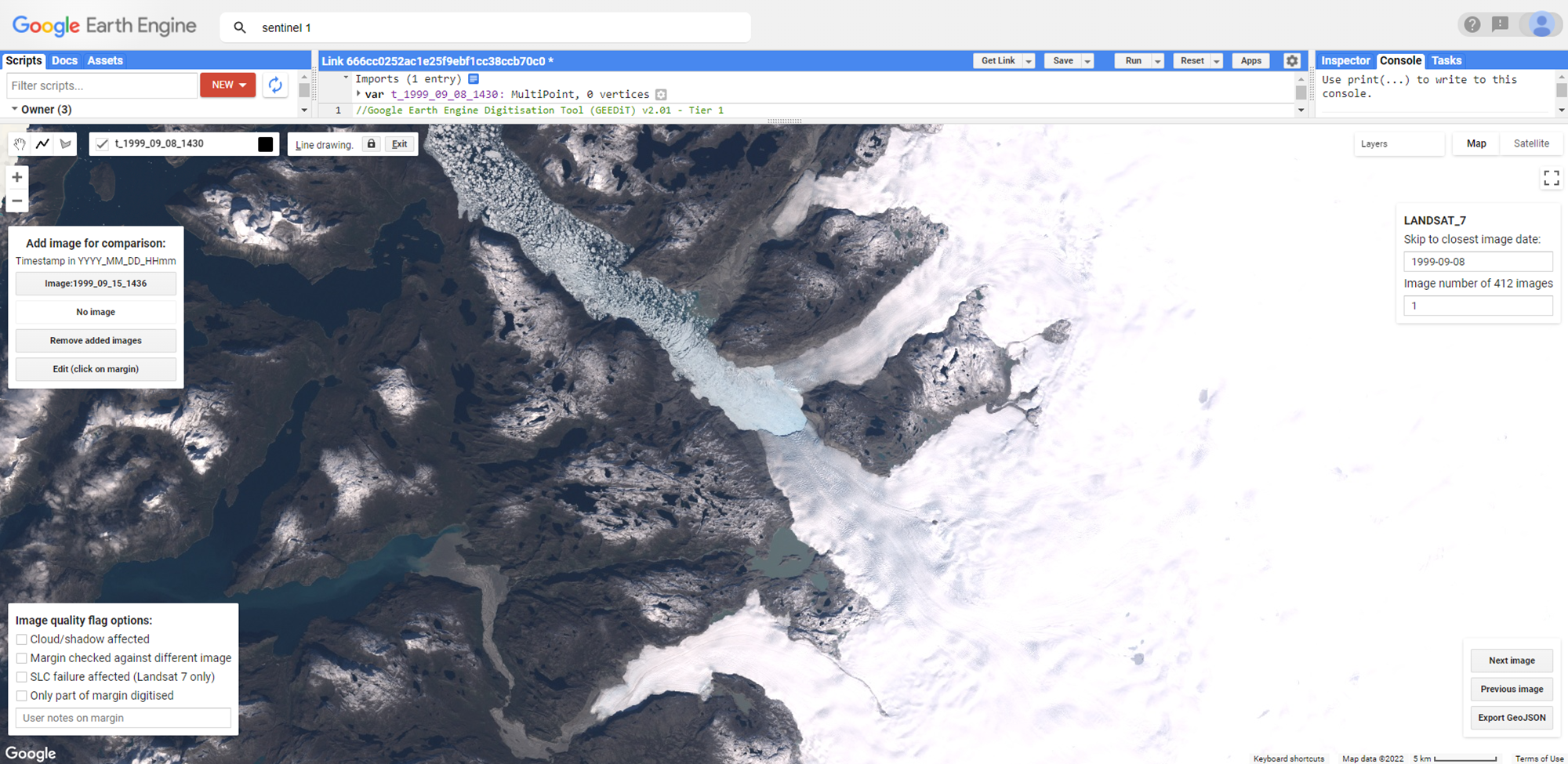
To visualize imagery once the desired options have been defined, zoom into your area of interest (in this case, southwest Greenland) and simply click on the map where imagery should be loaded. Once this is done, an “Imagery loading” panel will appear while GEEDiT collates all imagery for the clicked location that satisfies the image selection options. If lots of imagery is returned, then it may take 30 seconds to a minute for the list of images to be obtained. Once GEEDiT has loaded this, the vector digitization screen will appear, and the earliest image available from the list will be visualized automatically (Fig. F5.4.3).

Section 2. GEEDiT Digitisation Interface

Section 2.1. Digitizing and Editing Margins and Features

The GEEDiT digitization interface will load and the first image will appear, providing you with multiple options to interact with vectors and imagery. However, if you wish to begin digitizing straight away, you can do so by clicking directly on the image, and double clicking to finish the final vertex of the feature or margin. By default, vectors will be digitized as a line. However you can also draw polygons by selecting this option from the top left of the screen.

Once vectors have been digitized, you may wish to modify or delete vectors where required. To do this, either click the edit button on the top left panel before clicking on the digitized margin that is to be changed, or press the keyboard escape key and click to select the margin (Fig. F5.4.4). The selected vector will show all digitized vertices as solid white circles, and the midpoints between vertices as semi-transparent circles. Any of these can be dragged using the cursor to modify the vector. If you want to delete the entire vector, press your keyboard’s Delete key.

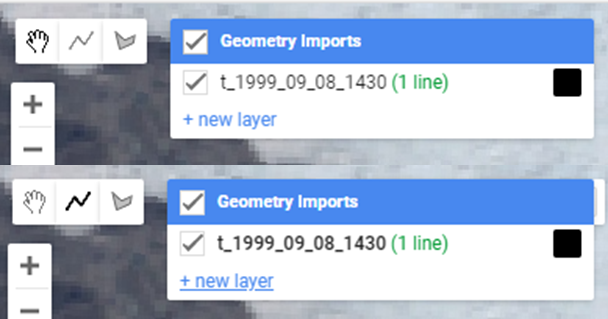
In order to begin digitizing again, hover your cursor over the geometry layer at the top left of the screen, and click on the relevant layer so that it changes from standard to bold typeface (Fig. F5.4.5). Do not use the “+ new layer” option.

You can then digitize multiple lines and/or polygons to individual images, and they will be saved in the geometry layer selected. The name of the geometry layer is given in the format t_YYYY_MM_DD_HHmm, also providing you with information as to the precise time and date that the source image was acquired.

Section 2.2. Moving Between Images

There are multiple options in GEEDiT for how you can move from the current image to the next. Options to move between images are contained in the two panels on the right-hand side of the screen (Fig. F5.4.6). Note that when a new image is loaded, the interface creates a new geometry layer for that image, and sets previous layers to be not visible on the map (though these can be easily visualized where comparison may be needed). The geometry layer related to the current image will be black, while vectors digitized from other imagery will be blue.

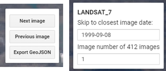
To move between images, the first option is to click Next image; if you do, the user interface will load image number 2 in the list. Similarly, the Previous image button will load the preceding image in the list where one is available. Try clicking Next image to bring up image number 2.

Other options to move between images are provided in the panel on the upper right of the screen (Fig. F5.4.6, right). This panel contains information on which satellite the image was acquired by, the date that the image was acquired, and the image number. The date and image number are contained within editable textboxes, and provide two different ways for moving to a new image.

The first option is to edit the text box containing the date of the current image (in YYYY-MM-DD format), and allows users to skip to the image in the list that is closest in time to the date that they define. Once the new date has been entered, the user should press the keyboard enter key to trigger the image to load. GEEDiT will then visualize the image that is closest to the user defined date, and update the value of the text box with the actual date of the image. The second option is to change the image number text box value, press enter, and then GEEDiT will load that image number from the list of images available. Try each of these options for yourself.

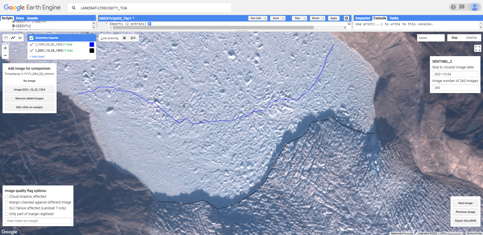
Section 2.3. Visualizing Previously Digitized Margins or Features on the Current Image

The geometries of each vector digitized from each image are retained as geometry layers in the digitization interface (Fig. F5.4.5). Consequently, you can revisualize previously digitized vectors on the current image by toggling the check boxes next to each geometry layer, providing a means to briefly check how or if a feature has changed between one date or another. In the user interface the margin relating to the current image will appear as black, while previously digitized vectors will appear as blue (Fig. F5.4.7). This functionality is not intended as a substitute for analysis, but a means for you to quickly check whether change has occurred, thus facilitating potential study site identification.

Section 2.4. Extra Functionality

GEEDiT provides the ability to compare between images, for interpreting subtle features in the current image. This functionality is contained in the top left panel of the digitization interface (Fig. F5.4.8).

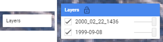
The options in this panel allows users to easily add the images immediately preceding and following the current image. Try clicking on these buttons to add imagery to the map, and use the Remove added images button to remove any imagery that has been added to leave only the original image visualized. To aid comparison between images, try using the image layer transparency slider bars contained in the map Layers dropdown in the top right of the digitization interface (Fig. F5.4.9).

When using this option take care to ensure that vectors are digitized directly from the current image only (in the case above, 1999-09-08) to ensure data consistency.

Section 2.5. Image Quality Flags

For some margins and features, it may be necessary to note problems that have impacted the quality of vector digitization. To aid in this, GEEDiT includes several quality flags for common issues. These are contained in the panel in the bottom left of the screen with information from these flags added to vector metadata upon export (Fig. F5.4.10).

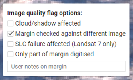
These quality flags help you to subsequently filter any vectors impacted by imagery issues that may affect the quality or accuracy of the vector digitization. These options are:

• Cloud/shadow affected: The user may wish to flag a vector as having been negatively impacted by cloud or shadow.
• Margin checked against different image: This flag is automatically checked when you add an image for comparison (see above and Fig. F5.4.8).
• SLC failure affected: This flag is automatically checked if margins from an image that is impacted by the Landsat 7 SLC failure is used (see Sect. 1, Landsat 7 description). You may wish to uncheck this box if vectors that are digitized from SLC failure affected imagery fall within areas that are not impacted by image data gaps.
• Only part of margin digitized: When it is only possible for you to digitize part of the full feature of interest, then this flag should be checked
• Text box for user notes: This text box provides the opportunity for you to provide brief notes (up to 256 characters) on the vectors digitized. These notes will be preserved in the exported data.

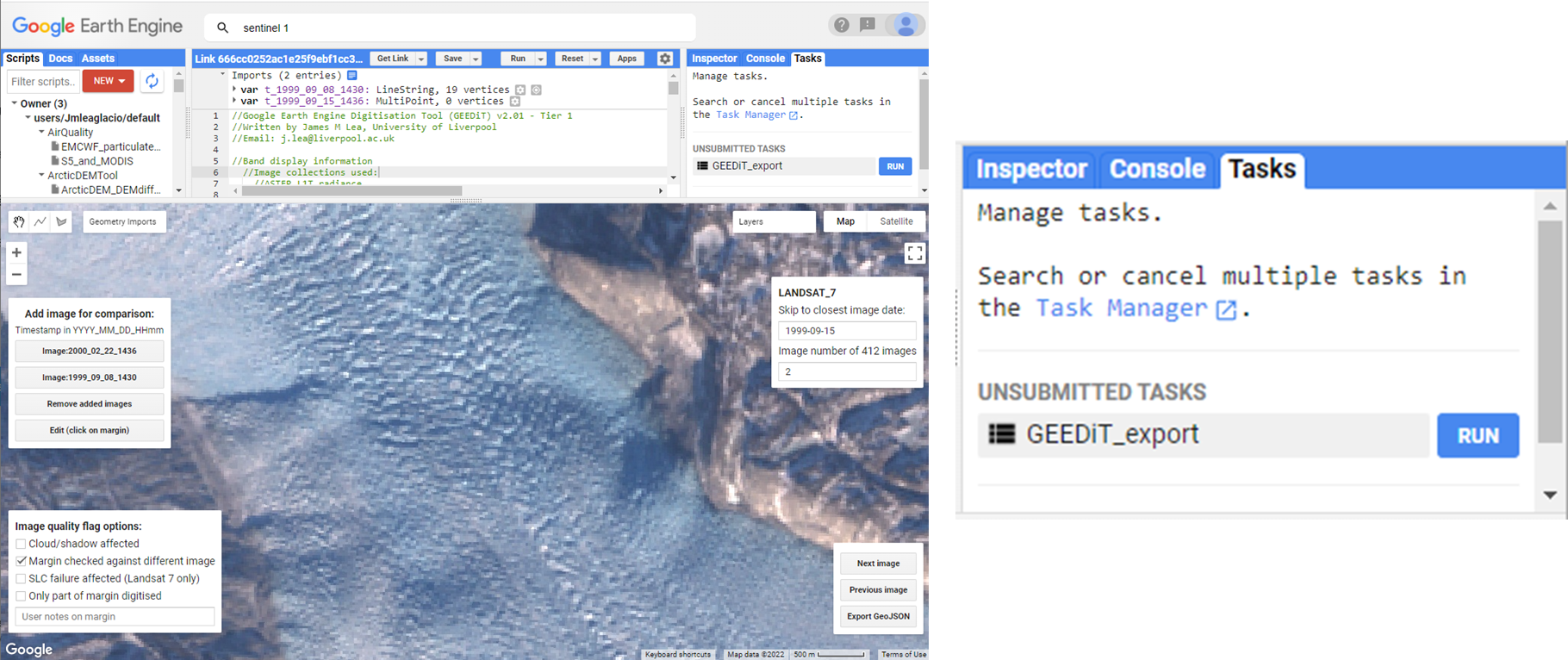
Section 2.6. Exporting Data

Once you have digitized all the vectors that you wish to, or you have reviewed enough imagery to automatically trigger an export task (see Sect. 1 and Fig. F5.4.2), you can export your digitized vectors to your Google Drive or to Earth Engine as an asset. To manually trigger an export task, try clicking the Export GeoJSON button in the bottom right panel shown on the screen (Fig. F5.4.6). It is important to note that just this step alone will not result in data being exported. To execute the export task, go to the Tasks tab next to the Earth Engine Code Editor. To access this, you may need to resize the map from the top of the screen to make this visible (Fig. F5.4.11).

To trigger the export, click the blue Run button in the Tasks tab. This will bring up the Earth Engine data export menu (Fig. F5.4.12). In this menu the user has the option to define the task name (note that this is not how the export will be saved, but how the name of the export task will appear in the Tasks tab), the folder in Google Drive where the exported file will be saved, the name of the exported file, and the format of the exported file. As default, the GeoJSON file format is selected, due to its capability of retaining both line and polygon vectors within the same file. If users have digitized only lines, or only polygons, it is possible to export these as shapefiles. However, if a user attempts to export a combination of lines and polygons as a single shapefile, this will fail. GeoJSON files can be easily imported into GIS platforms such as QGIS or ArcGIS, while their consistent file structure also assists coding-based analysis.

Section 3. Making GEEDiT Fit Your Own Purposes (Advanced)

Section 3.1. Changing Default Image Band Combinations and Visualization Ranges

GEEDiT has been designed to visualize, where possible, true color satellite imagery at the highest possible spatial resolution. However, for some applications, margins or features may be identified more easily using different satellite image band combinations or minimum/maximum image data ranges. Where this is necessary, there are two options available to you:

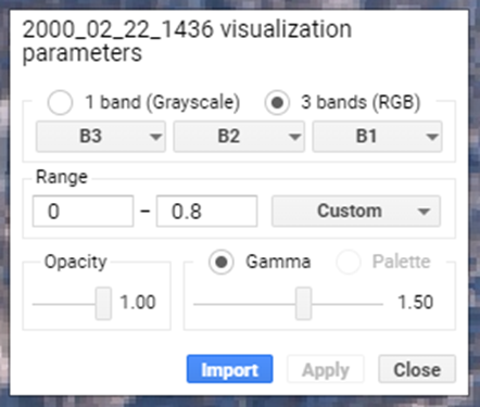
1. After an image has been visualized, try manually editing the image bands and data range by hovering over the map Layers menu and the image to be edited (Fig. F5.4.9), before clicking the Gear icon that appears next to the image name. This will bring up image visualization options that allow editing of the image band combination, in addition to a variety of options to define the minimum/maximum data values. Try exploring some of the options that this provides, and to implement the changes, click the Apply button to re-visualize the image using the new band and minimum/maximum visualization options (Fig. F5.4.13). However, note that this will not change the default visualization options in GEEDiT, and if you go to the next image, the default visualization options will be restored (see below).

2. Changing GEEDiT’s default image band combinations and/or minimum/maximum values requires direct editing GEEDiT’s code within the GEE code editor and making changes to the imVisParams variable (Fig. F5.4.14; L420-428 in GEEDiT v2.02). This will allow you to change the default band combinations and other image visualization options for each satellite. Once changes have been made, click the Run button above the Code Editor for the changes to take effect. If you are unfamiliar with Earth Engine or JavaScript, any changes in GEEDiT’s code should be undertaken with care, given that any small formatting errors could result in the tool failing to run or resulting in unexpected behavior. It is suggested that users take care not to delete any brackets, colons, commas, or inverted commas when editing these visualization options. Note that while Sentinel-1 has the HH band selected as default, in practice this is not frequently used, as some Sentinel-1 images do not contain this band.

Section 3.2. Filtering Image Lists by Other Image Metadata

The GEEDiT user interface is intended to provide a simple means by which margins and features can be digitized from satellite imagery. It is purposely not designed to provide comprehensive image filtering options so as to retain an intuitive, straightforward user experience. However, it is possible to make additions to GEEDiT’s code that allow users to filter image collections by other image metadata.

For example, in order to find imagery that highlights margins or features using shadows, users may wish to only digitize from optical imagery where the sun angle at the time of image acquisition does not exceed a given value. This can be achieved by adding lines that will filter imagery by metadata values to L326-387 (GEEDiT v2.02). If you wish to do this, then care should be taken to ensure that the correct image metadata names are used, and also note that these metadata names can vary between satellite platforms. More information on the metadata available for each satellite platform can be found in the relevant links in Sect. 1 where the satellites are described. For more information on how to filter image collections, see Chap. F4.1.

Section 3.3. Changing Image Collections Used in GEEDiT

For optical satellites, GEEDiT uses real-time TOA image collections for Landsat and Sentinel-2, as these provide the highest numbers of images (see Sect. 1). However, in some circumstances it may be more appropriate to use different image collections that are available in Earth Engine (e.g., surface reflectance imagery that has been calibrated for atmospheric conditions at the time of acquisition). If this is the case, you can change GEEDiT’s code to access this imagery as default by updating the image collection paths used to access satellite data (contained between L326-387 in GEEDiT v2.02).

The different image collections available within Earth Engine can be explored using the search bar at the top of the screen above the user interface, and users should read information relating to each image collection carefully to ensure that the data will be appropriate for the task that they wish to undertake. Users should also replace paths in a “like for like” fashion (i.e., Landsat 8 TOA replaced with Landsat 8 SR), as otherwise this will result in incorrect metadata being appended to digitized vectors when they are exported. To do this, try replacing the Landsat 8 TOA collection with the path name for a Landsat 8 Surface Reflectance image collection that can be found using the search bar. Once you have made the changes, click Run for them to take effect.

Section 3.4. Saving Changes to GEEDiT Defaults for Future Use

If you have edited GEEDiT to implement your own defaults, then you can save this for future use rather than needing to change these settings each time you open GEEDiT. This can be easily done by clicking the Save button at the top of the Code Editor, allowing you to access your edited GEEDiT version via the Scripts tab to the left of the Code Editor. For more information on the Earth Engine interface, see Chapter F1.0.

Synthesis

You should now be familiar with the GEEDiT user interface, its functionality, and options to modify default visualization parameters of the tool.

Assignment 1. Visualize imagery from your own area of interest and digitize multiple features or margins using polygons and lines.

Assignment 2. Export these data and visualize them in an offline environment (e.g., QGIS, ArcMap, Matplotlib), and view the metadata associated with each vector. Think how these metadata may prove useful when post-processing your data.

Assignment 3. Try modifying the GEEDiT code to change the tool’s default visualization parameters for Landsat 8 imagery to highlight the features that you are interested in digitizing (e.g., band combinations and value ranges to highlight water, vegetation etc.).

Assignment 4. Using information about the wavelengths detected by different bands for other optical satellites, change the default visualization parameters for Landsat 4, 5, and 7, and Sentinel-2 so that they are consistent with the modified Landsat 8 visualization parameters.

Conclusion

This chapter has covered the background to the Earth surface margin and feature digitization tool GEEDiT. It provides an introduction to the imagery used within GEEDiT and some of the considerations to take into account when digitizing from these, in addition to a walkthrough of how to use GEEDiT and its functionality. The final section provides some information on how to edit GEEDiT for bespoke purposes, though you are encouraged to do this with care. You will be able to confidently use the interface, and conceptually understand how the tool operates.

Feedback

To review this chapter and make suggestions or note any problems, please go now to bit.ly/EEFA-review. You can find summary statistics from past reviews at bit.ly/EEFA-reviews-stats.

References

Cloud-Based Remote Sensing with Google Earth Engine. (n.d.). CLOUD-BASED REMOTE SENSING WITH GOOGLE EARTH ENGINE. https://www.eefabook.org/

Cloud-Based Remote Sensing with Google Earth Engine. (2024). In Springer eBooks. https://doi.org/10.1007/978-3-031-26588-4

Boothroyd RJ, Williams RD, Hoey TB, et al (2021) Applications of Google Earth Engine in fluvial geomorphology for detecting river channel change. Wiley Interdiscip Rev Water 8:e21496. https://doi.org/10.1002/wat2.1496

Brough S, Carr JR, Ross N, Lea JM (2019) Exceptional retreat of Kangerlussuaq Glacier, East Greenland, between 2016 and 2018. Front Earth Sci 7:123. https://doi.org/10.3389/feart.2019.00123

Chander G, Markham BL, Helder DL (2009) Summary of current radiometric calibration coefficients for Landsat MSS, TM, ETM+, and EO-1 ALI sensors. Remote Sens Environ 113:893–903. https://doi.org/10.1016/j.rse.2009.01.007

Fahrner D, Lea JM, Brough S, et al (2021) Linear response of the Greenland ice sheet’s tidewater glacier terminus positions to climate. J Glaciol 67:193–203. https://doi.org/10.1017/jog.2021.13

Field HR, Armstrong WH, Huss M (2021) Gulf of Alaska ice-marginal lake area change over the Landsat record and potential physical controls. Cryosphere 15:3255–3278. https://doi.org/10.5194/tc-15-3255-2021

Kochtitzky W, Copland L, Painter M, Dow C (2020) Draining and filling of ice-dammed lakes at the terminus of surge-type Dań Zhùr (Donjek) Glacier, Yukon, Canada. Can J Earth Sci 57:1337–1348. https://doi.org/10.1139/cjes-2019-0233

Lea JM (2018) The Google Earth Engine Digitisation Tool (GEEDiT) and the Margin change Quantification Tool (MaQiT) – Simple tools for the rapid mapping and quantification of changing Earth surface margins. Earth Surf Dyn 6:551–561. https://doi.org/10.5194/esurf-6-551-2018

Scheingross JS, Repasch MN, Hovius N, et al (2021) The fate of fluvially-deposited organic carbon during transient floodplain storage. Earth Planet Sci Lett 561:116822. https://doi.org/10.1016/j.epsl.2021.116822

Tuckett PA, Ely JC, Sole AJ, et al (2019) Rapid accelerations of Antarctic Peninsula outlet glaciers driven by surface melt. Nat Commun 10:1–8. https://doi.org/10.1038/s41467-019-12039-2