Cloud-Based Remote Sensing with Google Earth Engine

Fundamentals and Applications

Part A1: Human Applications

This Part covers some of the many Human Applications of Earth Engine. It includes demonstrations of how Earth Engine can be used in agricultural and urban settings, including for sensing the built environment and the effects it has on air composition and temperature. This Part also covers the complex topics of human health, illicit deforestation activity, and humanitarian actions.

Chapter A1.8: Monitoring Gold Mining Activity Using SAR

Authors

Lucio Villa, Sidney Novoa, Milagros Becerra, Andréa Puzzi Nicolau, Karen Dyson, Karis Tenneson, John Dilger

Overview

The expansion of gold mining has had a large impact on the rainforests of the Amazon over the last decades. To take just one example, it has affected both the biodiversity and the lives of local people in the Madre de Dios region of southeastern Peru. In this chapter, we will review a methodology developed to generate early warnings of deforestation based on the use of synthetic aperture radar (SAR) images. First, we will identify the Sentinel-1 images suitable for the construction of a time series of preprocessed datasets. Second, we will run a change detection analysis based on a statistical analysis of the Sentinel-1 images (Canty et al. 2019). Finally, we will show the steps to follow in the post-processing stage by filtering information with forest / non-forest and bodies of water datasets.

Learning Outcomes

• Selecting and creating a multitemporal SAR mosaic.
• Generating SAR change detection based on a statistical analysis of Sentinel-1 images.
• Post-processing of alerts generated by filtering maximum area patches and information of forest/non-forest and water bodies.

Helps if you know how to:

• Import, filter, and visualize images (Part F1).
• Work with time-series data in Earth Engine (Part F4).
• Write a function and map it over an ImageCollection (Chap. F4.0).
• Use the require function to load code from existing modules (Chap. F6.1).
• Export results to assets (Chap. F6.2).

Github Code link for all tutorials

This code base is collection of codes that are freely available from different authors for google earth engine.

Github Source

Introduction to Theory

Accelerated demand for natural resources has transformed the Amazon rainforest into a new economic frontier that generates commodities such as agricultural products, livestock, and more recently, minerals, especially gold (RAISG 2020). In Peru, illegal gold mining is a serious problem that affects local populations in the southeastern region of Madre de Dios (Yard et al. 2012, Asner and Tupayachi 2017, Alvarez-Berrios et al. 2021). According to Caballero et al. (2018), it has led to the deforestation of about 1,000 km2 of rainforest, affecting protected areas, Indigenous communities, and sustainable management areas. Gold mining is carried out throughout the year, even during the rainy season.

Optical Earth-observation satellites have played a very important role in monitoring gold-mining deforestation in recent years. Madre de Dios is one of the few tropical regions in the world for which there is well-documented information on annual forest loss due to this deforestation driver (Asner et al. 2013, Asner and Tupayachi 2017, Caballero et al. 2018, Nicolau et al. 2019, Csillick and Asner 2020, Alarcón Aguirre et al. 2021). However, these resources do not reveal the progress of illegal mining during the rainy season and at other times when the optical images are obscured by clouds. This reduces the window of opportunity to know the dynamics of the activity and guide actions to control the advance of deforestation.

Satellite-based SAR sensors obtain information throughout the entire year thanks to the ability of microwaves to penetrate cloud cover (Ballere et al. 2021, Nicolau et al. 2021). Therefore, we are able to capture changes due to gold mining expansion with SAR data from the European Space Agency (ESA) Sentinel-1 C-band satellite. In this chapter, we will look at a successful example of how to process radar images to generate early warnings of gold-mining deforestation.

Practicum

SAR sensors transmit microwave signals at an oblique angle and measure the backscattered portion of the signal in order to analyze features on the surface. Unlike optical sensors, which are passive, SAR is an active instrument with its own source of illumination, and it is one of the few sensing instruments that allows full control of the signal polarization on both the transmit and receive paths. The majority of today’s SAR sensors are linearly polarized, and transmit horizontally and/or vertically polarized wave forms (i.e., SAR bands can be VV, VH, HV, or HH). While interpreting optical imagery is similar to interpreting a photograph, interpreting SAR data requires a different way of thinking, in that the signal is instead responsive in complex ways to surface characteristics such as structure and moisture. More information about the theory and concepts behind SAR is available in the SAR Handbook (Flores-Anderson et al. 2019).

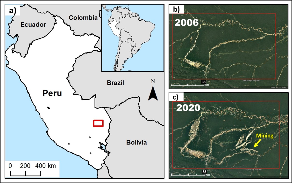
The area of study for this chapter is the region surrounding a mining corridor located in Madre de Dios in the southern Peruvian Amazon (Fig. A1.8.1).

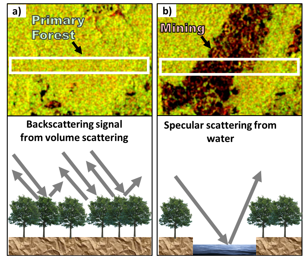
Alluvial gold mining exploitation generates changes in the radar backscattering mechanism over forested areas, since it involves deforestation, removal of topsoil, excavation, and the use of water for the extraction of gold from the loose sediment. Fig. A1.8.2 shows the changes in SAR Sentinel-1 images and a radar backscattering mechanism before (Fig. A1.8.2a) and after (Fig. A1.8.2b) the impact of alluvial gold mining activity.

Therefore, you will learn how to use SAR Sentinel-1 time series to detect changes generated by alluvial gold mining activities in forested areas.

The first step is to create a SAR mosaic for a given period of time and orbit pass. Then, we will apply the omnibus Q-test algorithm to generate change alerts from the SAR Sentinel-1 time series. Finally, we will filter and eliminate potential false positive alerts coming from other activities with the same temporal pattern as the mining activity (e.g., natural forest loss by river expansion or water over bare soil during the rainy season).

Section 1. Creating a Single SAR Mosaic

We will use ESA’s Sentinel-1 dual-polarized (VV+VH) in descending orbit pass to create a single SAR mosaic over the area of study. Sentinel-1 SAR Ground Range Detected (GRD) data (Fig. A1.8.3) is stored in Earth Engine in two formats: logarithmic scale (dB) and the original values (power scale named as FLOAT). We will use the latter since mathematical operations should not be applied into data on a logarithmic scale. The Sentinel-1 dataset is composed of Level-1 SAR amplitude multi-look images preprocessed according to the following steps: orbit metadata update, removal of border and thermal noise, radiometric calibration and terrain correction.

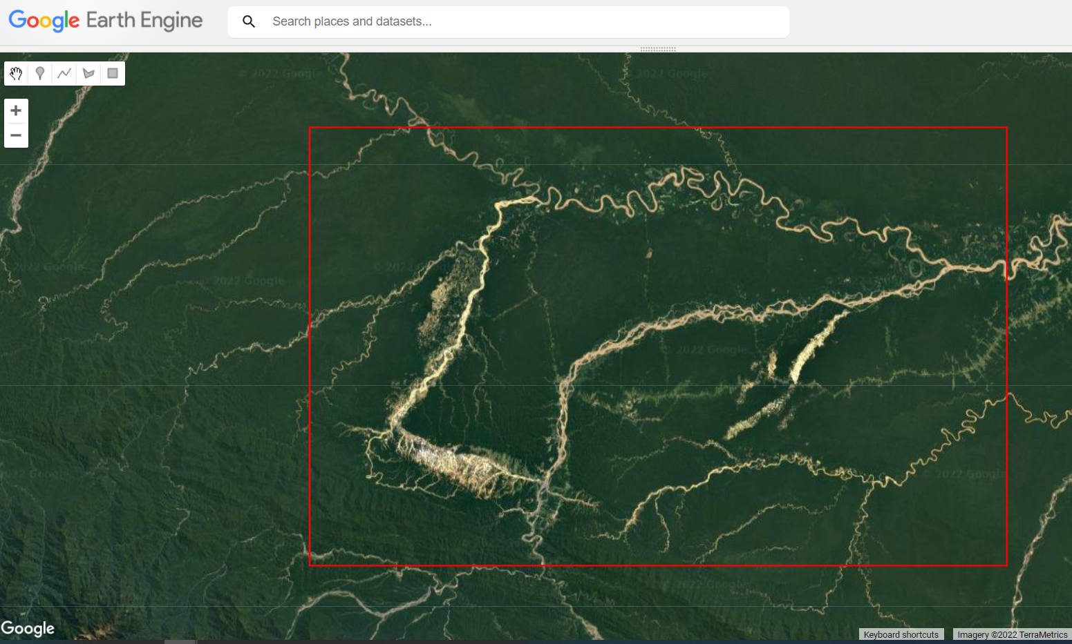
Copy and paste the code below to define the area of study (Fig. A1.8.1), convert this vector to a boundary image, and add it to the map (Fig. A1.8.4).

Next, copy and paste the code below to define two functions, maskAngle and getCollection. The first function masks sections of SAR images acquired at an incidence angle less than 31 or greater than 45 degrees. The second function filters the Sentinel-1 imagery to a specific period of time, region of interest, and orbit pass. Note that the Sentinel-1 GRD dataset is imported inside the second function.

Copy and paste the code below to import the Sentinel-1 collection, define time variables (a list of dates) and the orbit pass variable, apply the functions, create a mosaic by using the mosaic function, and clip the mosaic to the study area.

Before adding the mosaic to the map, it’s important to scale the values to a logarithmic scale (log10().multiply(10.0)). The parameters of visualization (sarVis) should be taken between 3 and -23 decibels (dB). Copy and paste the code below to do so and to add the mosaic to the map (Fig. A1.8.5). The code creates a scaled image and draws it using visualization parameters set through trial and error.

Code Checkpoint A18a. The book’s repository contains a script that shows what your code should look like at this point.

Question 1. How many bands (polarizations) does Sentinel-1 have over the area of study?

Question 2. Using the Inspector tool, explore the values from the VV and VH bands over different land covers. Which one do you think is better able to detect forested areas?

Section 2. Creating a SAR Mosaic Time Series

We will reuse most of the code from Section 1, only changing the period of time and not applying the mosaic function just yet. Start this section by opening the following code checkpoint.

Code Checkpoint A18b. The book’s repository contains a script to use to begin this section. You will need to start with that script and paste code below into it.

Expand the SAR ImageCollection in the Console and note that it is composed of 30 elements. To create a time series of mosaics, we need to define two additional functions (getDates and mosaicSAR). The first function converts the format of the date from milliseconds to format 'YYYY-MM-dd'. The second function filters the SAR ImageCollection using the list of dates and generates a mosaic. The result is an ImageCollection of mosaics per date. Copy and paste the code below to define these two functions.

Now, copy and paste the code below to generate a list of dates without duplicate elements (i.e., where there are images from the same dates in the collection, we only keep one). We avoid duplicates by using the ee.List.distinct and the getDates functions, and output an ImageCollection of mosaics per date.

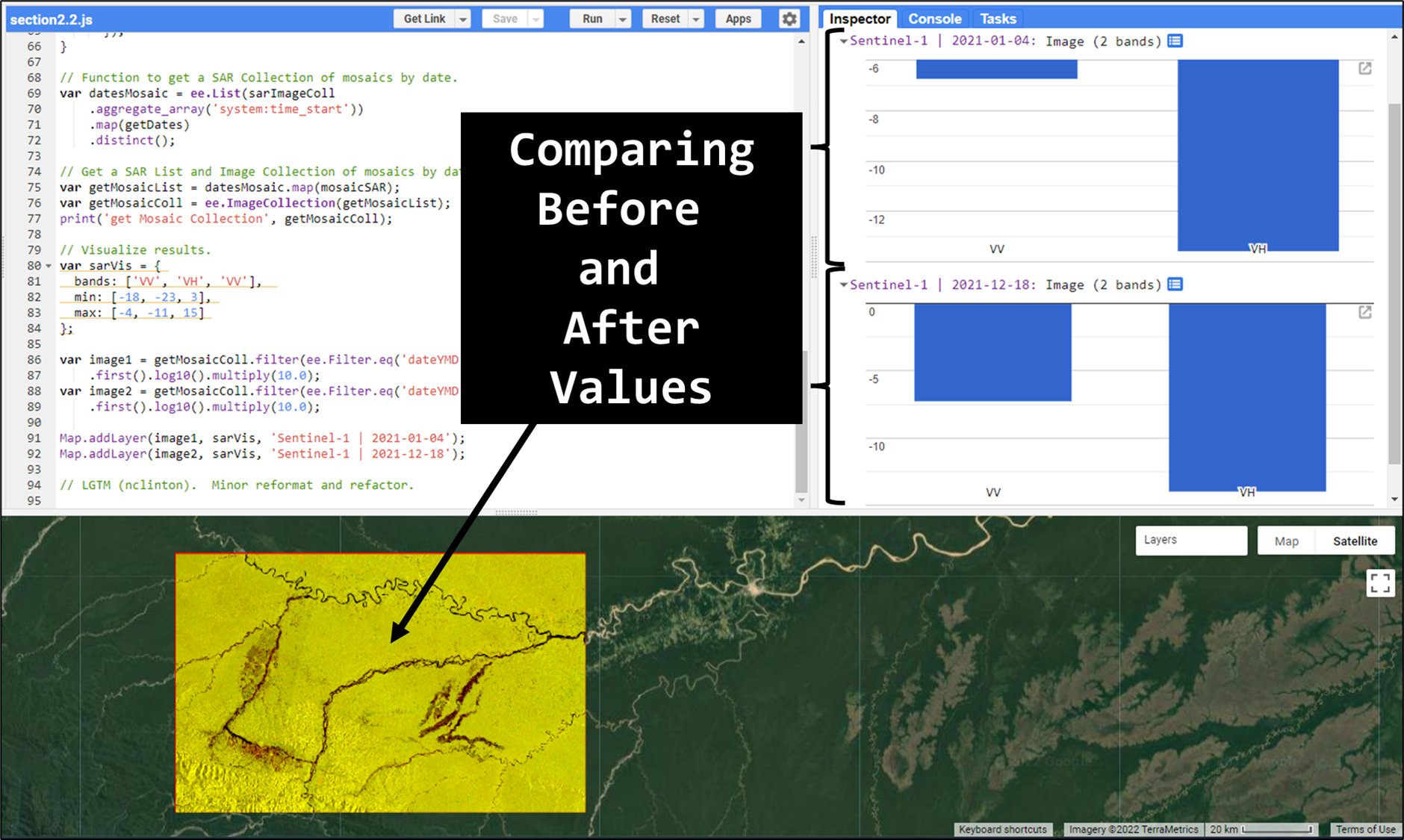
Finally, copy and paste the code below to set the visualization parameter (sarVis) and add two SAR mosaics filtered by the date of acquisition as an example (one from 2021-01-04 and the other from 2021-12-18; Fig. A1.8.6).

Note that we applied the logarithmic scale for visualization purposes. Zoom in and switch between the layers to note the differences between the images.

Code Checkpoint A18c. The book’s repository contains a script that shows what your code should look like at this point.

Question 3. How many images were taken by Sentinel-1 over the area of study between 2018-01-01 and 2020-01-01?

Question 4. Using the Inspector tool, explore the temporal changes of the values from VV and VH bands over new mining areas.

Section 3. Generate SAR Change Detection

There are different methods for detecting changes using SAR data. In this case, we will use a SAR change detection method based on Canty et al. (2020).

This methodology allows us to identify changes for a series of “k” uncorrelated SAR images using a pixel-based omnibus likelihood ratio test statistic Q for covariance matrices (∑i, i=1. . . k), based on a Wishart distribution. The Q test is defined by

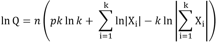
Where Xi=nΣ* (with Σ* being the maximum likelihood estimate of the covariance matrices Σi), “n” the number of looks and “p” the dimensionality of the covariance matrices (with p=2 for dual polarización SAR data). The | ∙ | denotes the determinant.

The Q test is an omnibus test statistic because it evaluates the equality of several covariance matrices simultaneously. Thus, this test statistic tests the null hypothesis (no change, H0) against alternative hypothesis (change, H1) using SAR time series pixel-based data and the level of significance (probability that the null hypothesis H0 is true, also known as p-value) estimated in each iteration.

In the first iteration, the first two first images in the time series are tested (null hypothesis of no change against the alternative of change):

If the Null hypothesis (H0) is not rejected, then the test continues including the values of the next image in the series:

However, if the null hypothesis is rejected in this iteration, then the interval of time for this change is labeled and the test is restarted from there.

The explanation of the Omnibus likelihood ratio test statistic is beyond the scope of this chapter but more details can be found in Canty et al. (2020).

The next steps correspond to obtaining a single change detection output image using the time series of mosaics generated in Section 2.

To do so, we will use modules adapted from the original JavaScript libraries by Canty et al (2020). Beginning from the last code checkpoint from Section 2, copy and paste the code below to import the adapted modules and define a variable that stores the number of images in our collection. This number will be used later on for visualization purposes.

Before applying the SAR change algorithm, we need to define the input parameters such as the significance and the reducer to be applied (median in this case). The result is an ee.Dictionary that contains several images: among these are cmap, smap, fmap, bmap. The cmap image shows the occurrence of the most recent significant change, smap shows the first significant change, fmap shows the frequency of significant changes, and bmap shows the interval in which each significant change occurred.

Copy and paste the code below to define such variables, apply the algorithm to the list of SAR mosaics (getMosaicList), and extract the results.

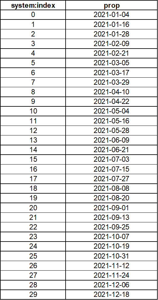
The values for cmap, smap, and bmap are numbers that correspond to dates. These are the dates that are stored in the datesMosaic list. For example, the pixel value of 0 corresponds to the first date (2021-01-04), the pixel value of 1 corresponds to the second date (2021-01-16), and so on (Fig. A1.8.7).

If we want to export the resulting images we need to also export the list of dates. To do so, we need to create a FeatureCollection since we can’t currently export lists directly in Earth Engine. Copy and paste the code below to create a FeatureCollection where each feature contains the date information as a property. We are also printing the dates in order to visualize the pixel-date association (expand the list on the Console to see it.)

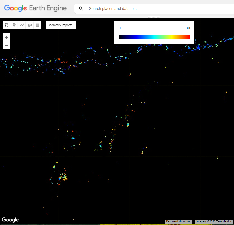
Now we can add the results to the map. Copy and paste the code below to define visualizations parameters, make a legend that associates date numbers with colors, and add the resulting images (Fig. A1.8.8).To load results faster, change the Map.centerObject function at the top of the script to Map.setCenter(-70.003, -12.849, 12)—we are zooming in to a specific area—and leave only the smap layer checked under the Layers panel.

Now, copy and paste the code below to export two items to Google Drive: fCollectionDates, the dates of SAR images processed (Fig. A1.8.7); and smap , the image of the first significant change (Fig. A1.8.8).

Code Checkpoint A18d. The book’s repository contains a script that shows what your code should look like at this point.

Question 5. What is the difference between the smap and cmap images?

Question 6. How does the FeatureCollection fCollectionDate relate to the change maps smap, cmap, and fmap?

Section 4. Filtering and Postprocessing Alerts

As explained earlier in the Practicum, the smap results need to be filtered in order to eliminate possible false positives. The false positives are associated with the forest loss due to river morphology and the presence of muddy water bodies (Fig. A1.8.2).

In this section, we will explore different options to filter false positives and, therefore, postprocess the results generated.

Like we did in previous sections, copy and paste the code below into a new script to import the study area and the exported smap image. Remember that our analysis covered 30 Sentinel-1 images from distinct dates.

Next, copy and paste the code below to import from the Earth Engine data catalog and add to the map all the sources of information for filtering false positives: Shuttle Radar Topography Mission (SRTM) digital elevation data, Hansen Global Forest Change data, and JRC Global Surface Water data (Fig. A1.8.9).

You can toggle these layers on and off, zoom in and out, and inspect pixel values to analyze them.

The SRTM elevation layer ('SRTM Elevation') and the slope ('SRTM Slope') derived from it with ee.Terrain.slope show red areas that correspond to an altitude over 1000 meters above sea level and a slope over 15 degrees, compared to blue areas, which are closer to sea level or to flat terrain. We chose these options because mining activity in this region is located in lowlands. Furthermore, the SAR Sentinel-1 data provided by Earth Engine are not radiometric-terrain corrected. So, steep slopes (>15 degrees) generate distortions in SAR images, and therefore, potential false changes between two or more images taken at different times.

The Hansen Global Forest Change data are composed of forested areas in 2000 (the 'treecover2000' band) and the forest loss between 2001 and 2020. In this sense, the binary layer 'Forest cover 2020' previously generated and added shows in green the forested areas updated until 2020, with all the non-forested and the forest loss between 2001-2020 areas masked.

The JRC Yearly Water Classification History data shows surface water extent and change between 1984 and 2020. The binary layer 'Water Bodies until 2020' previously added shows in blue the water bodies’ maximum extent between 1984 and 2020. Non-water bodies are shown in black.

Note that alluvial mining expansion pattern in the study area is associated with primary forest loss, and the appearance of new surface water patches (Fig. A1.8.2).

Now, we will filter the false positives based on thresholds. We will mask any pixel in smap marked as change over areas greater than 1000 meters above sea level, slope greater than 15 degrees according to the SRTM data (classified as forest until 2020 by the Hansen data), and that are not classified as water bodies by the JRC dataset. Copy and paste below to add the filtered results to the map.

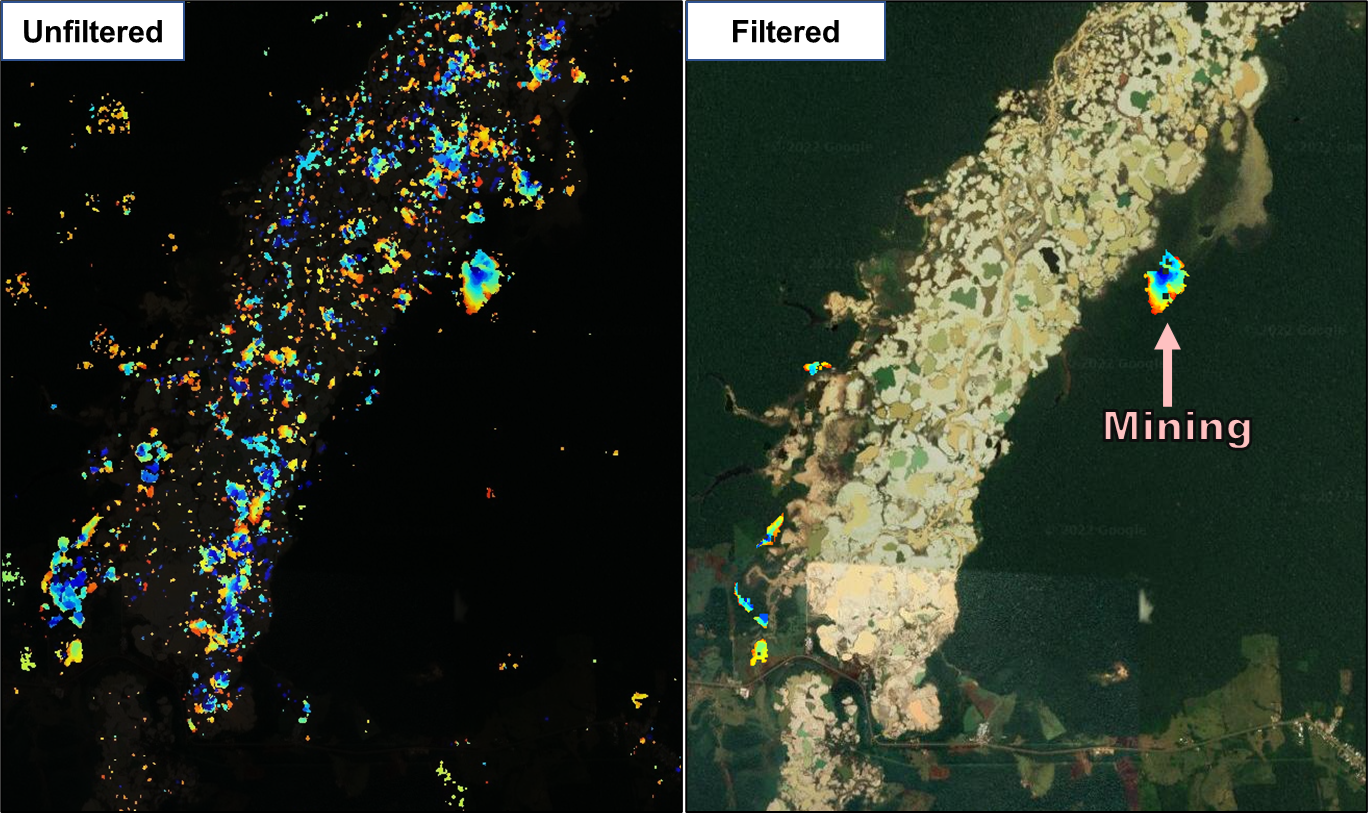
We can still improve the results a bit more. Copy and paste the code below to define and apply a function that eliminates small pixel patches and isolated pixels. We do this because we know that in this area, mining activities occur in areas of at least 0.5 hectares.

Turn off all the other layers to visualize the filtered result. By analyzing the results without the filters and with the filters, we can see that we eliminated most of the false positives (Fig. A1.8.10).

Finally, we can export the outcome. Copy and paste the code below to export to the Drive.

Code Checkpoint A18e. The book’s repository contains a script that shows what your code should look like at this point.

Synthesis

In this chapter, we mapped the changes generated by the alluvial mining activity over a forested area and between a period of time using Sentinel-1 SAR time series. For this, we separated the methodology into three steps. First, we were able to build a time series from Sentinel-1 mosaics. Second, we estimate all the changes based on the omnibus Q-test change detection algorithm. Finally, we filter the detected changes  based on existing forest/non-forest, water bodies, and elevation data, and a minimum mapping unit in order to retrieve the changes generated by the alluvial mining activity only.

Now, it’s your turn to explore the use of the methodology.

Assignment 1. In this chapter we applied the methodology for a given SAR orbit. Describe how we could identify the different SAR orbits over a specific area of study.

Assignment 2. Describe whether these alerts, which are generated by a change detection algorithm, are different for the ascending or descending orbit over our area of study.

Conclusion

In this chapter, you have learned how to analyze the changes generated by alluvial mining activity over forested areas based on the application of a SAR change detection methodology. This is possible because of the significant impact generated by this activity over the environment (that is, the deforestation and the use of water in the alluvial gold wash machine) that is reflected in the backscatter signal of SAR data. This methodology can be applied to other study cases since a good understanding of the principles of change detection has been achieved in this chapter and complemented by chapters in part F4.

Feedback

To review this chapter and make suggestions or note any problems, please go now to bit.ly/EEFA-review. You can find summary statistics from past reviews at bit.ly/EEFA-reviews-stats.

References

Aguirre GA, Robles RRC, Duarez FMG, et al (2021) Dinámica de la pérdida de bosques en el sureste de la Amazonia peruana: Un estudio de caso en Madre de Dios. Ecosistemas 30:2175. https://doi.org/10.7818/ECOS.2175

Álvarez-Berríos N, L’Roe J, Naughton-Treves L (2021) Does formalizing artisanal gold mining mitigate environmental impacts? Deforestation evidence from the Peruvian Amazon. Environ Res Lett 16:64052. https://doi.org/10.1088/1748-9326/abede9

Asner GP, Llactayo W, Tupayachi R, Luna ER (2013) Elevated rates of gold mining in the Amazon revealed through high-resolution monitoring. Proc Natl Acad Sci USA 110:18454–18459. https://doi.org/10.1073/pnas.1318271110

Asner GP, Tupayachi R (2017) Accelerated losses of protected forests from gold mining in the Peruvian Amazon. Environ Res Lett 12:94004. https://doi.org/10.1088/1748-9326/aa7dab

Ballère M, Bouvet A, Mermoz S, et al (2021) SAR data for tropical forest disturbance alerts in French Guiana: Benefit over optical imagery. Remote Sens Environ 252:112159. https://doi.org/10.1016/j.rse.2020.112159

Bourbigot M, Johnsen H, Piantanida R, Hajduch G (2021) Sentinel-1 Product Specification for products generated with IPF 3.4.0. CLS S-1 Mission Perform. Cent. pp. 186

Caballero Espejo J, Messinger M, Román-Dañobeytia F, et al (2018) Deforestation and forest degradation due to gold mining in the Peruvian Amazon: A 34-year perspective. Remote Sens 10:1903. https://doi.org/10.20944/preprints201811.0113.v1

Canty MJ, Nielsen AA, Conradsen K, Skriver H (2020) Statistical analysis of changes in Sentinel-1 time series on the Google Earth Engine. Remote Sens 12:46. https://doi.org/10.3390/rs12010046

Csillik O, Asner GP (2020) Near-real time aboveground carbon emissions in Peru. PLoS One 15:e0241418. https://doi.org/10.1371/journal.pone.0241418

Flores-Anderson AI, Herndon KE, Thapa RB, Cherrington E (2019) The SAR Handbook: Comprehensive Methodologies for Forest Monitoring and Biomass Estimation

Fröjse L (2014) Unsupervised change detection using multi-temporal SAR data: A case study of Arctic sea ice. KTH: Royal Institute of Technology

Gorelick N, Hancher M, Dixon M, et al (2017) Google Earth Engine: Planetary-scale geospatial analysis for everyone. Remote Sens Environ 202:18–27. https://doi.org/10.1016/j.rse.2017.06.031

Kellndorfer J, Flores-Anderson AI, Herndon KE, Thapa RB (2019) Using SAR data for mapping deforestation and forest degradation. SAR Handbook Compr Methodol For Monit Biomass Estim ServirGlobal Hunstville, AL, USA 65–79. https://doi.org/10.25966/68c9-gw82

Nicolau AP, Flores-Anderson A, Griffin R, et al (2021) Assessing SAR C-band data to effectively distinguish modified land uses in a heavily disturbed Amazon forest. Int J Appl Earth Obs Geoinf 94:102214. https://doi.org/10.1016/j.jag.2020.102214

Nicolau AP, Herndon K, Flores-Anderson A, Griffin R (2019) A spatial pattern analysis of forest loss in the Madre de Dios region, Peru. Environ Res Lett 14:124045. https://doi.org/10.1088/1748-9326/ab57c3

Proisy C, Mougin E, Fromard F, Rudant JP (1998) Télédétection radar des mangroves de Guyane Française. Séminaire Télédétection Végétation, Montpellier, Fr 1996-11-26, Photo interprétation 36:26

RAISG (2020) Amazonia Under Pressure. https://atlas2020.amazoniasocioambiental.org/en. Accessed 25 Feb 2022

Richards JA (2009) Remote Sensing with Imaging Radar. Springer

Rignot EJM, van Zyl JJ (1993) Change detection techniques for ERS-1 SAR data. IEEE Trans Geosci Remote Sens 31:896–906. https://doi.org/10.1109/36.239913

Yard EE, Horton J, Schier JG, et al (2012) Mercury exposure among artisanal gold miners in Madre de Dios, Peru: A cross-sectional study. J Med Toxicol 8:441–448. https://doi.org/10.1007/s13181-012-0252-0