Human Applications

Health Applications

Previous
Next

Cloud-Based Remote Sensing with Google Earth Engine

Fundamentals and Applications


Part A1: Human Applications


This Part covers some of the many Human Applications of Earth Engine. It includes demonstrations of how Earth Engine can be used in agricultural and urban settings, including for sensing the built environment and the effects it has on air composition and temperature. This Part also covers the complex topics of human health, illicit deforestation activity, and humanitarian actions.


 Chapter A1.6: Health Applications


Author

Dawn Nekorchuk


Overview

The purpose of this chapter is to demonstrate how Google Earth Engine may be used to support modeling and forecasting of vector-borne infectious diseases such as malaria. In doing so, the chapter will also show how Earth Engine may be used to gather data for subsequent analyses outside of Earth Engine, the results of which can then also be brought back into Earth Engine.

We will be calculating and exporting data of remotely-sensed environmental variables: precipitation, temperature, and a vegetation water index. These factors can impact mosquito life cycles, malaria parasites, and transmission dynamics. These data can then be used in R for modeling and forecasting malaria in the Amhara region of Ethiopia, using the Epidemic Prognosis Incorporating Disease and Environmental Monitoring for Integrated Assessment (EPIDEMIA) system, developed by the EcoGRAPH research group at the University of Oklahoma.

Learning Outcomes

  • Extracting and calculating malaria-relevant variables from existing data sets: precipitation, temperature, and wetness.
  • Importing satellite data and filtering for images over a region and time period.
  • Joining two data products to get additional quality information.
  • Computing zonal summaries of the calculated variables for elements in a FeatureCollection.

Helps if you know how to:

  • Import images and image collections, filter, and visualize (Part F1).
  • Perform basic image analysis: select bands, compute indices, create masks (Part F2).
  • Use expressions to perform calculations on image bands (Chap. F3.1).
  • Write a function and map it over an ImageCollection (Chap. F4.0).
  • Mask cloud, cloud shadow, snow/ice, and other undesired pixels (Chap. F4.3).
  • Flatten a table for export to CSV (Chap. F5.0).
  • Use reduceRegions to summarize an image with zonal statistics in irregular shapes (Chap. F5.0, Chap. F5.2).
  • Write a function and map it over a FeatureCollection (Chap. F5.1, Chap. F5.2).

Github Code link for all tutorials

This code base is collection of codes that are freely available from different authors for google earth engine.

Github Source


Introduction to Theory

Vector-borne diseases cause more than 700,000 deaths per year, of which approximately 400,000 are due to malaria, a parasitic infection spread by Anopheles mosquitoes (World Health Organization 2018, 2020). The WHO estimates that there were around 229 million clinical cases of malaria worldwide in 2019 (WHO 2020). Environmental factors including temperature, humidity, and rainfall are known to be important determinants of malaria risk as these affect mosquito and parasite development and life cycles, including larval habitats, mosquito fecundity, growth rates, mortality, and Plasmodium parasite development rates within the mosquito vector (Franklinos et al. 2019, Jones 2008, Wimberly et al. 2021).

Data from Earth-observing satellites can be used to monitor spatial and temporal changes in these environmental factors (Ford et al. 2009). These data can be incorporated into disease modeling, usually as lagged functions, to help develop early warning systems for forecasting outbreaks (Wimberly et al. 2021, 2022). Accurate forecasts would allow limited resources for prevention and control to be more efficiently and effectively targeted at appropriate locations and times (WHO 2018).

To implement near-real-time forecasting, meteorological and climatic data must be acquired, processed, and integrated on a regular and frequent basis. Over the past 10 years, the Epidemic Prognosis Incorporating Disease and Environmental Monitoring for Integrated Assessment (EPIDEMIA) project has developed and tested a malaria forecasting system that integrates public health surveillance with monitoring of environmental and climate conditions. Since 2018 the environmental data has been acquired using Earth Engine scripts and apps (Wimberly et al. 2022). In 2019 a local team at Bahir Dar University in Ethiopia had been using EPIDEMIA with near-real-time epidemiological data to generate weekly malaria early warning reports in the Amhara region of Ethiopia.

In this example, we are looking at near-real-time environmental conditions that affect disease vectors and human transmission dynamics. On longer time scales, issues such as climate change can alter vector-borne disease transmission cycles and the geographic distributions of various vector and host species (Franklinos 2019). More broadly, health applications involving Earth Engine data likely align with a One Health approach to complex health issues. Under One Health, a core assumption is that environmental, animal, and human health are inextricably linked (Mackenzie and Jeggo 2019).


Practicum 

The goal of the practicum is to create a download of three environmental variables:

  1. Precipitation
  2. Mean land surface temperature (LST)
  3. Normalized Difference Water Index (NDWI) spectral index.

These downloads will be zonal summaries based on our uploaded shapefile of woredas (districts) in the Amhara region of Ethiopia.

The practicum is an extract from the longer Retrieving Environmental Analytics for Climate and Health (REACH) Earth Engine script (developed by Dr. Michael C. Wimberly and Dr. Dawn Nekorchuk) used in the EPIDEMIA project (Dr. Michael C. Wimberly, PI). This script also has a more advanced user interface for the user to request date ranges for the download of data. Links to this script and related apps can be found in the “For Further Reading” section of this book.

Section 1. Data Import

To start, we need to import the data we will be working with. The first item is an external asset of our study area—these are woredas in the Amhara region of Ethiopia. The four that follow are remotely sensed data that we will be processing:

  • The Integrated Multi-satellite Retrievals for GPM (IMERG) rainfall estimates from Global Precipitation Measurement (GPM) v6
  • Terra Land Surface Temperature and Emissivity 8-Day Global 1km
  • MODIS Nadir BRDF (Bidirectional Reflectance Distribution Function) Adjusted Reflectance Daily 500m
  • MODIS BRDF-Albedo Quality Daily 500m

// Section 1: Data Import
var woredas=ee.FeatureCollection(
   
'projects/gee-book/assets/A1-6/amhara_woreda_20170207');
// Create region outer boundary to filter products on.
var amhara=woredas.geometry().bounds();
var gpm=ee.ImageCollection('NASA/GPM_L3/IMERG_V06');
var LSTTerra8=ee.ImageCollection('MODIS/061/MOD11A2')
   
// Due to MCST outage, only use dates after this for this script.
   .
filterDate('2001-06-26', Date.now());
var brdfReflect=ee.ImageCollection('MODIS/006/MCD43A4');
var brdfQa=ee.ImageCollection('MODIS/006/MCD43A2');

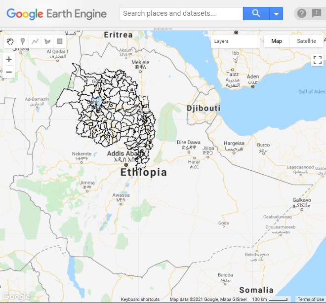
We can take a look at the woreda boundaries by adding the following code to draw it onto the map (Fig. A1.6.1). See Chap. F5.3 for more information on visualizing feature collections.

// Visualize woredas with black borders and no fill.
// Create an empty image into which to paint the features, cast to byte.
var empty=ee.Image().byte();
// Paint all the polygon edges with the same number and width.
var outline=empty.paint({
   featureCollection: woredas,
   color:
1,
   width:
1
});
// Add woreda boundaries to the map.
Map.setCenter(38, 11.5, 7);
Map.addLayer(outline,{
   palette:
'000000'
},
'Woredas');

Code Checkpoint A16a. The book’s repository contains a script that shows what your code should look like at this point.

Fig. A1.6.1 Woreda (district) boundaries in the Amhara region of Ethiopia

Section 2. Date Preparation

The user will be requesting the date range for the summarized data, and it is expected that they will be looking for near-real-time data. Different data products that we are using have different data lags, and some data may not be available in the user-requested date range. We will want to get the last available data date so we can properly create and name our export datasets.

We need daily data, but the LST data are in 8-day composites. For this, we will assign the 8-day composite value to each of the eight days in the range. This means we also need to acquire the 8-day composite value that covers the requested start date (i.e., the previous image).

// Section 2: Handling of dates

// 2.1 Requested start and end dates.
var reqStartDate=ee.Date('2021-10-01');
var reqEndDate=ee.Date('2021-11-30');

// 2.2 LST Dates
// LST MODIS is every 8 days, and a user-requested date will likely not match.
// We want to get the latest previous image date,
//  i.e. the date the closest, but prior to, the requested date.
// We will filter later.
// Get date of first image.
var LSTEarliestDate=LSTTerra8.first().date();
// Filter collection to dates from beginning to requested start date.
var priorLstImgCol=LSTTerra8.filterDate(LSTEarliestDate,
   reqStartDate);
// Get the latest (max) date of this collection of earlier images.
var LSTPrevMax=priorLstImgCol.reduceColumns({
   reducer:
ee.Reducer.max(),
   selectors: [
'system:time_start']
});
var LSTStartDate=ee.Date(LSTPrevMax.get('max'));
print('LSTStartDate', LSTStartDate);

// 2.3 Last available data dates
// Different variables have different data lags.
// Data may not be available in user range.
// To prevent errors from stopping script,
//  grab last available (if relevant) & filter at end.

// 2.3.1 Precipitation
// Calculate date of most recent measurement for gpm (of all time).
var gpmAllMax=gpm.reduceColumns(ee.Reducer.max(), [
   
'system:time_start'
]);
var gpmAllEndDateTime=ee.Date(gpmAllMax.get('max'));
// GPM every 30 minutes, so get just date part.
var gpmAllEndDate=ee.Date.fromYMD({
   year: gpmAllEndDateTime.
get('year'),
   month: gpmAllEndDateTime.
get('month'),
   day: gpmAllEndDateTime.
get('day')
});

// If data ends before requested start, take last data date,
// otherwise use requested date.
var precipStartDate=ee.Date(gpmAllEndDate.millis()
   .
min(reqStartDate.millis()));
print('precipStartDate', precipStartDate);

// 2.3.2 BRDF
// Calculate date of most recent measurement for brdf (of all time).
var brdfAllMax=brdfReflect.reduceColumns({
   reducer:
ee.Reducer.max(),
   selectors: [
'system:time_start']
});
var brdfAllEndDate=ee.Date(brdfAllMax.get('max'));
// If data ends before requested start, take last data date,
// otherwise use the requested date.
var brdfStartDate=ee.Date(brdfAllEndDate.millis()
   .
min(reqStartDate.millis()));
print('brdfStartDate', brdfStartDate);
print('brdfEndDate', brdfAllEndDate);

Code Checkpoint A16b. The book’s repository contains a script that shows what your code should look like at this point.

Question 1. Explore the earliest date of LST images you get if you do not specifically acquire the previous image. The following code may be useful:

var naiveLstFilter=LSTTerra8.filterDate(reqStartDate, reqEndDate);
var naiveLstStart=naiveLstFilter.reduceColumns({
   reducer:
ee.Reducer.min(),
   selectors: [
'system:time_start']
});
var naiveLstStartDate=ee.Date(naiveLstStart.get('min'));
print('naiveLstStartDate', naiveLstStartDate);

Question 2. Try changing the requested dates to closer to the current date to see how the dates for the different data products adjust. If you have a narrow window (1–2 weeks), you may find that some data products do not have any data available for the requested time period yet.

Section 3. Precipitation

Now we will calculate our precipitation variable for the appropriate date range and then perform a zonal summary (see Chap. F5.2) of our woredas.

Section 3.1. Precipitation Filtering and Dates

Using the dates when data actually exists in the user-requested date range, we create a list of dates for which we will calculate our variable.


// Section 3: Precipitation

// Section 3.1: Precipitation filtering and dates

// Filter gpm by date, using modified start if necessary.
var gpmFiltered=gpm
   .
filterDate(precipStartDate, reqEndDate.advance(1, 'day'))
   .
filterBounds(amhara)
   .
select('precipitationCal');

// Calculate date of most recent measurement for gpm
// (in the modified requested window).
var gpmMax=gpmFiltered.reduceColumns({
   reducer:
ee.Reducer.max(),
   selectors: [
'system:time_start']
});
var gpmEndDate=ee.Date(gpmMax.get('max'));
var precipEndDate=gpmEndDate;
print('precipEndDate ', precipEndDate);

// Create a list of dates for the precipitation time series.
var precipDays=precipEndDate.difference(precipStartDate, 'day');
var precipDatesPrep=ee.List.sequence(0, precipDays, 1);

function makePrecipDates(n){
   
return precipStartDate.advance(n, 'day');
}
var precipDates=precipDatesPrep.map(makePrecipDates);

Section 3.2. Calculate Daily Precipitation

In this section, we will map a function over our filtered FeatureCollection (gpmFiltered) to calculate the total daily rainfall per day. In this product, precipitation in millimeters per hour is recorded every half hour, so we will sum the day and divide by two.

// Section 3.2: Calculate daily precipitation

// Function to calculate daily precipitation:
function calcDailyPrecip(curdate){
   curdate=
ee.Date(curdate);
   
var curyear=curdate.get('year');
   
var curdoy=curdate.getRelative('day', 'year').add(1);
   
var totprec=gpmFiltered
       .
filterDate(curdate, curdate.advance(1, 'day'))
       .
select('precipitationCal')
       .
sum()
       
//every half-hour
       .
multiply(0.5)
       .
rename('totprec');

   
return totprec
       .
set('doy', curdoy)
       .
set('year', curyear)
       .
set('system:time_start', curdate);
}
// Map function over list of dates.
var dailyPrecipExtended=
   
ee.ImageCollection.fromImages(precipDates.map(calcDailyPrecip));

// Filter back to the original user requested start date.
var dailyPrecip=dailyPrecipExtended
   .
filterDate(reqStartDate, precipEndDate.advance(1, 'day'));

Section 3.3. Summarize Daily Precipitation by Woreda

In the last section for precipitation, we will calculate a zonal summary, a mean, of the rainfall per woreda and flatten for export as a CSV. The exports (of all variables) will be all done in Sect. 7.

// Section 3.3: Summarize daily precipitation by woreda

// Filter precip data for zonal summaries.
var precipSummary=dailyPrecip
   .
filterDate(reqStartDate, reqEndDate.advance(1, 'day'));

// Function to calculate zonal statistics for precipitation by woreda.
function sumZonalPrecip(image){
   
// To get the doy and year,
   
// convert the metadata to grids and then summarize.
   
var image2=image.addBands([
       image.
metadata('doy').int(),
       image.
metadata('year').int()
   ]);
   
// Reduce by regions to get zonal means for each county.
   
var output=image2.select(['year', 'doy', 'totprec'])
       .
reduceRegions({
           collection: woredas,
           reducer:
ee.Reducer.mean(),
           scale:
1000
       });
   
return output;
}
// Map the zonal statistics function over the filtered precip data.
var precipWoreda=precipSummary.map(sumZonalPrecip);
// Flatten the results for export.
var precipFlat=precipWoreda.flatten();

Code Checkpoint A16c. The book’s repository contains a script that shows what your code should look like at this point.

Section 4. Land Surface Temperature

We will follow a similar pattern of steps for land surface temperatures, though first we will calculate the variable (mean LST). Then we will calculate the daily values and summarize them by woreda.

Section 4.1. Calculate LST Variables

We will use the daytime and nighttime observed values to calculate a mean value for the day. We will use the quality layers to mask out poor-quality pixels. Working with the bitmask below, we are taking advantage of the fact that bits 6 and 7 are at the end, so the rightShift(6) just returns these two. Then we check if they are less than or equal to 2, meaning average LST error <=3k (see MODIS documentation for the meaning of each element in the bit sequence). For more information on how to use bitmasks in other situations, see Chap. F4.3. To convert the pixel values, we will use the scaling factor in the data product (0.2) and convert from Kelvin to Celsius values (−273.15). See Chap. F1.5, about Heat Islands, for another example using LST data. 

// Section 4: Land surface temperature

// Section 4.1: Calculate LST variables

// Filter Terra LST by altered LST start date.
// Rarely, but at the end of the year if the last image is late in the year
//  with only a few days in its period, it will sometimes not grab
//  the next image. Add extra padding to reqEndDate and
//  it will be trimmed at the end.
var LSTFiltered=LSTTerra8
   .
filterDate(LSTStartDate, reqEndDate.advance(8, 'day'))
   .
filterBounds(amhara)
   .
select('LST_Day_1km', 'QC_Day', 'LST_Night_1km', 'QC_Night');

// Filter Terra LST by QA information.
function filterLstQa(image){
   
var qaday=image.select(['QC_Day']);
   
var qanight=image.select(['QC_Night']);
   
var dayshift=qaday.rightShift(6);
   
var nightshift=qanight.rightShift(6);
   
var daymask=dayshift.lte(2);
   
var nightmask=nightshift.lte(2);
   
var outimage=ee.Image(image.select(['LST_Day_1km',
       
'LST_Night_1km'
   ]));
   
var outmask=ee.Image([daymask, nightmask]);
   
return outimage.updateMask(outmask);
}
var LSTFilteredQa=LSTFiltered.map(filterLstQa);

// Rescale temperature data and convert to degrees Celsius (C).
function rescaleLst(image){
   
var LST_day=image.select('LST_Day_1km')
       .
multiply(0.02)
       .
subtract(273.15)
       .
rename('LST_day');
   
var LST_night=image.select('LST_Night_1km')
       .
multiply(0.02)
       .
subtract(273.15)
       .
rename('LST_night');
   
var LST_mean=image.expression(
       
'(day + night) / 2',{
           
'day': LST_day.select('LST_day'),
           
'night': LST_night.select('LST_night')
       }
   ).
rename('LST_mean');
   
return image.addBands(LST_day)
       .
addBands(LST_night)
       .
addBands(LST_mean);
}
var LSTVars=LSTFilteredQa.map(rescaleLst);

Section 4.2. Calculate Daily LST

Now, using a mapped function over our filtered collection, we will calculate a daily value from the 8-day composite value by assigning each of the eight days the value of the composite. We will also filter to our user-requested dates, as data exists in that range.

// Section 4.2: Calculate daily LST

// Create list of dates for time series.
var LSTRange=LSTVars.reduceColumns({
   reducer:
ee.Reducer.max(),
   selectors: [
'system:time_start']
});
var LSTEndDate=ee.Date(LSTRange.get('max')).advance(7, 'day');
var LSTDays=LSTEndDate.difference(LSTStartDate, 'day');
var LSTDatesPrep=ee.List.sequence(0, LSTDays, 1);

function makeLstDates(n){
   
return LSTStartDate.advance(n, 'day');
}
var LSTDates=LSTDatesPrep.map(makeLstDates);

// Function to calculate daily LST by assigning the 8-day composite summary
// to each day in the composite period:
function calcDailyLst(curdate){
   
var curyear=ee.Date(curdate).get('year');
   
var curdoy=ee.Date(curdate).getRelative('day', 'year').add(1);
   
var moddoy=curdoy.divide(8).ceil().subtract(1).multiply(8).add(
       
1);
   
var basedate=ee.Date.fromYMD(curyear, 1, 1);
   
var moddate=basedate.advance(moddoy.subtract(1), 'day');
   
var LST_day=LSTVars
       .
select('LST_day')
       .
filterDate(moddate, moddate.advance(1, 'day'))
       .
first()
       .
rename('LST_day');
   
var LST_night=LSTVars
       .
select('LST_night')
       .
filterDate(moddate, moddate.advance(1, 'day'))
       .
first()
       .
rename('LST_night');
   
var LST_mean=LSTVars
       .
select('LST_mean')
       .
filterDate(moddate, moddate.advance(1, 'day'))
       .
first()
       .
rename('LST_mean');
   
return LST_day
       .
addBands(LST_night)
       .
addBands(LST_mean)
       .
set('doy', curdoy)
       .
set('year', curyear)
       .
set('system:time_start', curdate);
}
// Map the function over the image collection
var dailyLstExtended=
   
ee.ImageCollection.fromImages(LSTDates.map(calcDailyLst));

// Filter back to original user requested start date
var dailyLst=dailyLstExtended
   .
filterDate(reqStartDate, LSTEndDate.advance(1, 'day'));

Section 4.3. Summarize Daily LST by Woreda

In the final section for LST, we will perform a zonal mean of the temperature to our woredas and flatten in preparation for export as CSV. The exports (of all variables) will be all done in Sect. 7.

// Section 4.3: Summarize daily LST by woreda

// Filter LST data for zonal summaries.
var LSTSummary=dailyLst
   .
filterDate(reqStartDate, reqEndDate.advance(1, 'day'));
// Function to calculate zonal statistics for LST by woreda:
function sumZonalLst(image) {
   
// To get the doy and year, we convert the metadata to grids
   
//  and then summarize.
   
var image2=image.addBands([
       image.
metadata('doy').int(),
       image.
metadata('year').int()
   ]);
   
// Reduce by regions to get zonal means for each county.
   
var output=image2
       .
select(['doy', 'year', 'LST_day', 'LST_night', 'LST_mean'])
       .
reduceRegions({
           collection: woredas,
           reducer:
ee.Reducer.mean(),
           scale:
1000
       });
   
return output;
}
// Map the zonal statistics function over the filtered LST data.
var LSTWoreda=LSTSummary.map(sumZonalLst);
// Flatten the results for export.
var LSTFlat=LSTWoreda.flatten();

Code Checkpoint A16d. The book’s repository contains a script that shows what your code should look like at this point.

Section 5. Spectral Index: NDWI

We will follow a similar pattern of steps for our spectral index, NDWI, as we did for precipitation and land surface temperatures: first, calculate the variable(s), then calculate the daily values, and finally summarize by woreda.

Section 5.1. Calculate NDWI

Here we will focus on NDWI, which we actively used in forecasting malaria. For examples on other indices, see Chap. F3.1. 

The MODIS MCD43A4 product contains simplified band quality information, and it is recommended to use the additional quality information in the MCD43A2 product for your particular application. We will join these two products to apply our selected quality information. (Note that we do not have to worry about snow in our study area.) For more information on joining image collections, see Chap. F4.9.


// Section 5: Spectral index NDWI

// Section 5.1: Calculate NDWI

// Filter BRDF-Adjusted Reflectance by date.
var brdfReflectVars=brdfReflect
   .
filterDate(brdfStartDate, reqEndDate.advance(1, 'day'))
   .
filterBounds(amhara)
   .
select([
           
'Nadir_Reflectance_Band1', 'Nadir_Reflectance_Band2',
           
'Nadir_Reflectance_Band3', 'Nadir_Reflectance_Band4',
           
'Nadir_Reflectance_Band5', 'Nadir_Reflectance_Band6',
           
'Nadir_Reflectance_Band7'
       ],
       [
'red', 'nir', 'blue', 'green', 'swir1', 'swir2', 'swir3']);

// Filter BRDF QA by date.
var brdfReflectQa=brdfQa
   .
filterDate(brdfStartDate, reqEndDate.advance(1, 'day'))
   .
filterBounds(amhara)
   .
select([
           
'BRDF_Albedo_Band_Quality_Band1',
           
'BRDF_Albedo_Band_Quality_Band2',
           
'BRDF_Albedo_Band_Quality_Band3',
           
'BRDF_Albedo_Band_Quality_Band4',
           
'BRDF_Albedo_Band_Quality_Band5',
           
'BRDF_Albedo_Band_Quality_Band6',
           
'BRDF_Albedo_Band_Quality_Band7',
           
'BRDF_Albedo_LandWaterType'
       ],
       [
'qa1', 'qa2', 'qa3', 'qa4', 'qa5', 'qa6', 'qa7', 'water']);

// Join the 2 collections.
var idJoin=ee.Filter.equals({
   leftField:
'system:time_end',
   rightField:
'system:time_end'
});
// Define the join.
var innerJoin=ee.Join.inner('NBAR', 'QA');
// Apply the join.
var brdfJoined=innerJoin.apply(brdfReflectVars, brdfReflectQa,
   idJoin);

// Add QA bands to the NBAR collection.
function addQaBands(image){
   
var nbar=ee.Image(image.get('NBAR'));
   
var qa=ee.Image(image.get('QA')).select(['qa2']);
   
var water=ee.Image(image.get('QA')).select(['water']);
   
return nbar.addBands([qa, water]);
}
var brdfMerged=ee.ImageCollection(brdfJoined.map(addQaBands));

// Function to mask out pixels based on QA and water/land flags.
function filterBrdf(image) {
   
// Using QA info for the NIR band.
   
var qaband=image.select(['qa2']);
   
var wband=image.select(['water']);
   
var qamask=qaband.lte(2).and(wband.eq(1));
   
var nir_r=image.select('nir').multiply(0.0001).rename('nir_r');
   
var swir2_r=image.select('swir2').multiply(0.0001).rename(
       
'swir2_r');
   
return image.addBands(nir_r)
       .
addBands(swir2_r)
       .
updateMask(qamask);
}
var brdfFilteredVars=brdfMerged.map(filterBrdf);

// Function to calculate spectral indices:
function calcBrdfIndices(image){
   
var curyear=ee.Date(image.get('system:time_start')).get('year');
   
var curdoy=ee.Date(image.get('system:time_start'))
       .
getRelative('day', 'year').add(1);
   
var ndwi6=image.normalizedDifference(['nir_r', 'swir2_r'])
       .
rename('ndwi6');
   
return image.addBands(ndwi6)
       .
set('doy', curdoy)
       .
set('year', curyear);
}
// Map function over image collection.
brdfFilteredVars=brdfFilteredVars.
map(calcBrdfIndices);

Section 5.2. Calculate Daily NDWI

Similar to the other variables, we will calculate a daily value and filter to our user-requested dates, as data exists in that range.

// Section 5.2: Calculate daily NDWI

// Create list of dates for full time series.
var brdfRange=brdfFilteredVars.reduceColumns({
   reducer:
ee.Reducer.max(),
   selectors: [
'system:time_start']
});
var brdfEndDate=ee.Date(brdfRange.get('max'));
var brdfDays=brdfEndDate.difference(brdfStartDate, 'day');
var brdfDatesPrep=ee.List.sequence(0, brdfDays, 1);

function makeBrdfDates(n){
   
return brdfStartDate.advance(n, 'day');
}
var brdfDates=brdfDatesPrep.map(makeBrdfDates);

// List of dates that exist in BRDF data.
var brdfDatesExist=brdfFilteredVars
   .
aggregate_array('system:time_start');

// Get daily brdf values.
function calcDailyBrdfExists(curdate){
   curdate=
ee.Date(curdate);
   
var curyear=curdate.get('year');
   
var curdoy=curdate.getRelative('day', 'year').add(1);
   
var brdfTemp=brdfFilteredVars
       .
filterDate(curdate, curdate.advance(1, 'day'));
   
var outImg=brdfTemp.first();
   
return outImg;
}
var dailyBrdfExtExists=
   
ee.ImageCollection.fromImages(brdfDatesExist.map(
       calcDailyBrdfExists));

// Create empty results, to fill in dates when BRDF data does not exist.
function calcDailyBrdfFiller(curdate){
   curdate=
ee.Date(curdate);
   
var curyear=curdate.get('year');
   
var curdoy=curdate.getRelative('day', 'year').add(1);
   
var brdfTemp=brdfFilteredVars
       .
filterDate(curdate, curdate.advance(1, 'day'));
   
var brdfSize=brdfTemp.size();
   
var outImg=ee.Image.constant(0).selfMask()
       .
addBands(ee.Image.constant(0).selfMask())
       .
addBands(ee.Image.constant(0).selfMask())
       .
addBands(ee.Image.constant(0).selfMask())
       .
addBands(ee.Image.constant(0).selfMask())
       .
rename(['ndvi', 'evi', 'savi', 'ndwi5', 'ndwi6'])
       .
set('doy', curdoy)
       .
set('year', curyear)
       .
set('system:time_start', curdate)
       .
set('brdfSize', brdfSize);
   
return outImg;
}
// Create filler for all dates.
var dailyBrdfExtendedFiller=
   
ee.ImageCollection.fromImages(brdfDates.map(calcDailyBrdfFiller));
// But only used if and when size was 0.
var dailyBrdfExtFillFilt=dailyBrdfExtendedFiller
   .
filter(ee.Filter.eq('brdfSize', 0));
// Merge the two collections.
var dailyBrdfExtended=dailyBrdfExtExists
   .
merge(dailyBrdfExtFillFilt);

// Filter back to original user requested start date.
var dailyBrdf=dailyBrdfExtended
   .
filterDate(reqStartDate, brdfEndDate.advance(1, 'day'));

Section 5.3. Summarize Daily Spectral Indices by Woreda

Lastly in our NDWI section, we will use the mean to summarize the values for each of the woredas and prepare for export by flattening the dataset. The exports (of all variables) will be all done in Sect. 7.

// Section 5.3: Summarize daily spectral indices by woreda

// Filter spectral indices for zonal summaries.
var brdfSummary=dailyBrdf
   .
filterDate(reqStartDate, reqEndDate.advance(1, 'day'));

// Function to calculate zonal statistics for spectral indices by woreda:
function sumZonalBrdf(image){
   
// To get the doy and year, we convert the metadata to grids
   
//  and then summarize.
   
var image2=image.addBands([
       image.
metadata('doy').int(),
       image.
metadata('year').int()
   ]);
   
// Reduce by regions to get zonal means for each woreda.
   
var output=image2.select(['doy', 'year', 'ndwi6'])
       .
reduceRegions({
           collection: woredas,
           reducer:
ee.Reducer.mean(),
           scale:
1000
       });
   
return output;
}

// Map the zonal statistics function over the filtered spectral index data.
var brdfWoreda=brdfSummary.map(sumZonalBrdf);
// Flatten the results for export.
var brdfFlat=brdfWoreda.flatten();

Code Checkpoint A16e. The book’s repository contains a script that shows what your code should look like at this point.

Question 3. Here we are only calculating NDWI, which is calculated from the near infrared (NIR) and shortwave infrared 2 (SWIR2) bands. If we wanted to calculate a vegetation index like the Normalized Difference Vegetation Index (NDVI), which bands would we need to add? Where in Sects. 5.1 through 5.3 would we need to add or select the raw bands and/or our new calculated band? Note: Fully implementing this is one of the synthesis challenges, so this is a good head start!

Section 6. Map Display

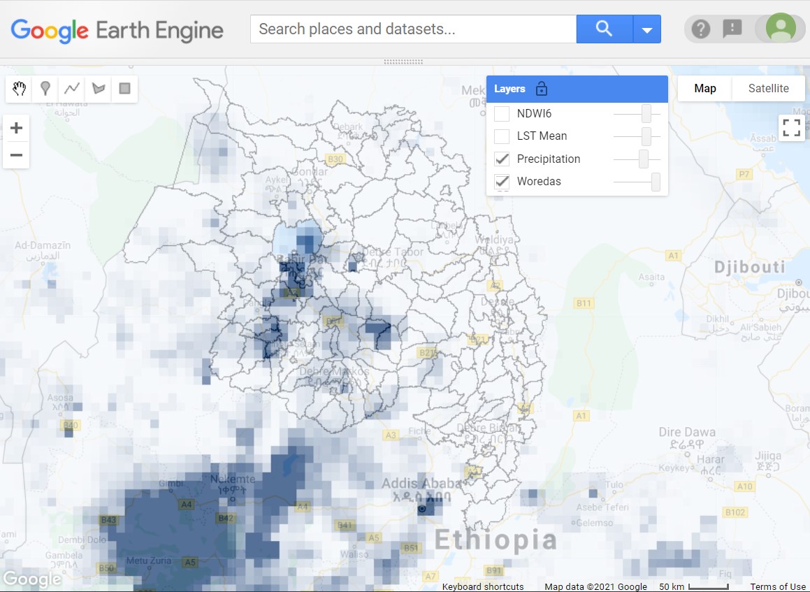
Here we will take a look at our calculated variables but prior to zonal summary (Fig. A1.6.2). The full user interface restricts the date to display within the requested range, so be mindful in the code below which date you choose to view (we set our time range here in Sect. 2.1).

// Section 6: Map display of calculated environmental variables
var displayDate=ee.Date('2021-10-01');

var precipDisp=dailyPrecip
   .
filterDate(displayDate, displayDate.advance(1, 'day'));
var brdfDisp=dailyBrdf
   .
filterDate(displayDate, displayDate.advance(1, 'day'));
var LSTDisp=dailyLst
   .
filterDate(displayDate, displayDate.advance(1, 'day'));

// Select the image (should be only one) from each collection.
var precipImage=precipDisp.first().select('totprec');
var LSTmImage=LSTDisp.first().select('LST_mean');
var ndwi6Image=brdfDisp.first().select('ndwi6');

// Palettes for environmental variable maps:
var palettePrecip=['f7fbff', '08306b'];
var paletteLst=['fff5f0', '67000d'];
var paletteSpectral=['ffffe5', '004529'];

// Add layers to the map.
// Show precipitation by default,
//  others hidden until users picks them from layers drop down.
Map.addLayer({
   eeObject: precipImage,
   visParams:{
       min:
0,
       max:
20,
       palette: palettePrecip
   },
   name:
'Precipitation',
   shown:
true,
   opacity:
0.75
});
Map.addLayer({
   eeObject: LSTmImage,
   visParams:{
       min:
0,
       max:
40,
       palette: paletteLst
   },
   name:
'LST Mean',
   shown:
false,
   opacity:
0.75
});
Map.addLayer({
   eeObject: ndwi6Image,
   visParams:{
       min:
0,
       max:
1,
       palette: paletteSpectral
   },
   name:
'NDWI6',
   shown:
false,
   opacity:
0.75
});

Code Checkpoint A16f. The book’s repository contains a script that shows what your code should look like at this point.

Fig. A1.6.2 Calculated total daily precipitation overlaid on woreda boundaries in the Amhara region of Ethiopia

Section 7. Exporting

Two important strengths of Google Earth Engine are the ability to gather and process the remotely sensed data all in the cloud, and to have the only download be a small text file ready to use in the forecasting software. Most of our partners on this project were experts in public health and did not have a remote sensing or programming background. We also had partners in areas of limited or unreliable internet connectivity. We needed something that could be easily usable by our users in these types of situations.

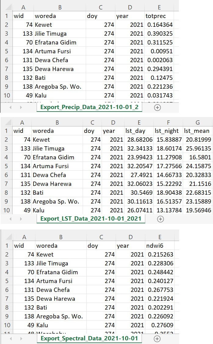
In this section, we will create small text CSV downloads for each of our three environmental factors prepared earlier. Each factor may have different data availability within the user’s requested range, and these dates will be added to the file name to indicate the actual date range of the downloaded data (Fig. A1.6.3).

// Section 7: Exporting

// 7.1 Export naming
var reqStartDateText=reqStartDate.format('yyyy-MM-dd').getInfo();

// Precipitation
var precipPrefix='Export_Precip_Data';
var precipLastDate=ee.Date(reqEndDate.millis()
   .
min(precipEndDate.millis()));
var precipSummaryEndDate=precipLastDate
   .
format('yyyy-MM-dd').getInfo();
var precipFilename=precipPrefix
   .
concat('_', reqStartDateText,
       
'_', precipSummaryEndDate);
// LST
var LSTPrefix='Export_LST_Data';
var LSTLastDate=ee.Date(reqEndDate.millis()
   .
min(LSTEndDate.millis()));
var LSTSummaryEndDate=LSTLastDate
   .
format('yyyy-MM-dd').getInfo();
var LSTFilename=LSTPrefix
   .
concat('_', reqStartDateText,
       
'_', LSTSummaryEndDate);
// BRDF
var brdfPrefix='Export_Spectral_Data';
var brdfLastDate=ee.Date(reqEndDate.millis()
   .
min(brdfEndDate.millis()));
var brdfSummaryEndDate=brdfLastDate
   .
format('yyyy-MM-dd').getInfo();
var brdfFilename=brdfPrefix
   .
concat('_', reqStartDateText,
       
'_', brdfSummaryEndDate);

// 7.2 Export flattened tables to Google Drive
// Need to click 'RUN in the Tasks tab to configure and start each export.
Export.table.toDrive({
   collection: precipFlat,
   description: precipFilename,
   selectors: [
'wid', 'woreda', 'doy', 'year', 'totprec']
});
Export.table.toDrive({
   collection: LSTFlat,
   description: LSTFilename,
   selectors: [
'wid', 'woreda', 'doy', 'year',
       
'LST_day', 'LST_night', 'LST_mean'
   ]
});
Export.table.toDrive({
   collection: brdfFlat,
   description: brdfFilename,
   selectors: [
'wid', 'woreda', 'doy', 'year', 'ndwi6']
});

Code Checkpoint A16g. The book’s repository contains a script that shows what your code should look like at this point.

In the Earth Engine Tasks tab, click Run to configure and start each export to Google Drive.

Fig. A1.6.3 Examples of the three CSV files returned from the script

Section 8. Importing and Viewing External Analyses Results

As mentioned at the start of the chapter, the environmental data obtained from Earth Engine can be used for infectious disease modeling and forecasting. The above Earth Engine code was written in support of EPIDEMIA, a software system based in the R language and computing environment for forecasting malaria, and was actively used in certain study pilot woredas in the Amhara region of Ethiopia. The R system consists of an R package—epidemiar—for generic functions and a companion R project for handling all the location-specific data and settings.

One of the main outputs of EPIDEMIA is the forecasted incidence of malaria in each woreda by week from one to eight (or more) weeks in advance. Using our publicly available demo project that uses synthetic data (not for use in epidemiological study), we created forecasts for week 32 of 2018 made eight weeks prior (“knowing” data up to week 24), and also added the observed incidence for comparison. (Note: dates and weeks follow International Organization for Standardization [ISO] standard 8601). These new data can be re-uploaded to Earth Engine for further analyses or exploration.

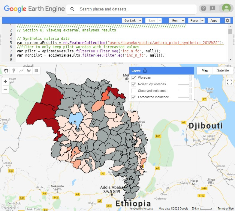
Starting a new script, you can use the Sect. 8 code that follows to visualize the pre-generated demo 2018W32 results (Fig. A1.6.4).  

// Section 8: Viewing external analyses results

// This is using *synthetic* malaria data.
// For demonstration only, not to be used for epidemiological purposes.
var epidemiaResults=ee.FeatureCollection(
   
'projects/gee-book/assets/A1-6/amhara_pilot_synthetic_2018W32'
);
// Filter to only keep pilot woredas with forecasted values.
var pilot=epidemiaResults
   .
filter(ee.Filter.neq('inc_n_fc', null));
var nonpilot=epidemiaResults
   .
filter(ee.Filter.eq('inc_n_fc', null));

Map.setCenter(38, 11.5, 7);

// Paint the pilot woredas with different colors for forecasted* incidence
// fc_n_inc here is the forecasted incidence (cut into factors)
// made on (historical) 2018W24 (i.e. 8 weeks in advance).
// * based on synthetic data for demonstration only.
// Incidence per 1000
// 1 : [0 - 0.25)
// 2 : [0.25 - 0.5)
// 3 : [0.5 - 0.75)
// 4 : [0.75 - 1)
// 5 : > 1

var empty=ee.Image().byte();
var fill_fc=empty.paint({
   featureCollection: pilot,
   color:
'inc_n_fc',
});
var palette=['fee5d9', 'fcae91', 'fb6a4a', 'de2d26', 'a50f15'];
Map.addLayer(
   fill_fc,{
       palette: palette,
       min:
1,
       max:
5
   },
   
'Forecasted Incidence'
);

// Paint the woredas with different colors for the observed* incidence.
// * based on synthetic data for demonstration only
var fill_obs=empty.paint({
   featureCollection: pilot,
   color:
'inc_n_obs',
});
var palette=['fee5d9', 'fcae91', 'fb6a4a', 'de2d26', 'a50f15'];
// Layer is off by default, users change between the two in the map viewer.
Map.addLayer(
   fill_obs,{
       palette: palette,
       min:
1,
       max:
5
   },
   
'Observed Incidence',
   
false
);

// Add gray fill for nonpilot woredas (not included in study).
var fill_na=empty.paint({
   featureCollection: nonpilot
});
Map.addLayer(
   fill_na, {
       palette:
'a1a9a8'
   },
   
'Non-study woredas'
);

// Draw borders for ALL Amhara region woredas.
var outline=empty.paint({
   featureCollection: epidemiaResults,
   color:
1,
   width:
1
});
// Add woreda boundaries to map.
Map.addLayer(
   outline, {
       palette:
'000000'
   },
   
'Woredas'
);

Code Checkpoint A16h. The book’s repository contains a script that shows what your code should look like at this point.

Fig. A1.6.4 Visualization of forecasted malaria incidence for week 32 of 2018 made during week 24 (an eight-week lead time). Malaria data is synthetic, for demonstration purposes only. The incidence has been categorized into five categories (from lighter to dark red): 0–0.25, 0.25–0.5, 0.5–0.75, 0.75–1, and greater than 1. Only woredas in the pilot project have values; the rest of the Amhara region is marked in gray fill. Another layer available to view is the observed (synthetic) incidence rate for 2018W32.

Synthesis

Assignment 1. Calculate other spectral indices: In this chapter, we only calculate and export the NDWI from the spectral data. Calculate another index, such as a vegetation index like NDVI, Soil Adjusted Vegetation Index (SAVI), or Enhanced Vegetation Index (EVI) to the calculations. Think about what bands you will need, how to calculate the index, and how to propagate the band through all the remaining processing steps (including exporting).

Assignment 2. Change location: In this chapter we obtained data for woredas in the Amhara region of Ethiopia. Upload or import a new shapefile of different locations and acquire environmental data for there instead. Remember that you will need to adjust any references to asset-specific fields (as we did here for “woreda”). See Chap. F5.0 for help with uploading assets, if needed.

Conclusion

In this chapter, we saw how Earth Engine can be used to acquire environmental data to support external analyses, such as forecasting of malaria, a vector-borne disease. An understanding of the biology of the vector (e.g., mosquito, tick), and how different environmental conditions can affect the disease system and transmission risk, will help identify environmental variables to investigate for use in mathematical modeling.

In this chapter we obtained data from three different satellite-based datasets: rainfall from IMERG/GPM, land surface temperature 8-day composite values from MODIS, and the calculation of spectral indices from MODIS bands. We saw how to perform zonal summaries to our location of interest, and download CSV files that are suitable for import into other programs for additional analyses.

This chapter shows the value of cloud computation and generating small downloads for use by professionals who may not have expertise in remote sensing or the computing resources that would otherwise be needed. Finally, we saw that the results of intermediate processing and work outside of Earth Engine can be re-imported for additional analyses within Earth Engine.      

Feedback

To review this chapter and make suggestions or note any problems, please go now to bit.ly/EEFA-review. You can find summary statistics from past reviews at bit.ly/EEFA-reviews-stats.

References

Cloud-Based Remote Sensing with Google Earth Engine. (n.d.). CLOUD-BASED REMOTE SENSING WITH GOOGLE EARTH ENGINE. https://www.eefabook.org/

Cloud-Based Remote Sensing with Google Earth Engine. (2024). In Springer eBooks. https://doi.org/10.1007/978-3-031-26588-4

Ford TE, Colwell RR, Rose JB, et al (2009) Using satellite images of environmental changes to predict infectious disease outbreaks. Emerg Infect Dis 15:1341–1346. https://doi.org/10.3201/eid/1509.081334

Franklinos LHV, Jones KE, Redding DW, Abubakar I (2019) The effect of global change on mosquito-borne disease. Lancet Infect Dis 19:e302–e312. https://doi.org/10.1016/S1473-3099(19)30161-6

Jones KE, Patel NG, Levy MA, et al (2008) Global trends in emerging infectious diseases. Nature 451:990–993. https://doi.org/10.1038/nature06536

Mackenzie JS, Jeggo M (2019) The one health approachwhy is it so important? Trop. Med. Infect. Dis. 4:88. https://doi.org/10.3390/tropicalmed4020088

Wimberly MC, de Beurs KM, Loboda T V., Pan WK (2021) Satellite observations and malaria: New opportunities for research and applications. Trends Parasitol 37:525–537. https://doi.org/10.1016/j.pt.2021.03.003

Wimberly MC, Nekorchuk DM, Kankanala RR (2022) Cloud-based applications for accessing satellite Earth observations to support malaria early warning. Sci Data 9:1–11. https://doi.org/10.1038/s41597-022-01337-y

World Health Organization (2018) Malaria surveillance, monitoring and evaluation: a reference manual. World Health Organization

World Health Organization (2020) World Malaria Report 2020: 20 years of global progress and challenges. World Health Organization


Previous
Next
MENU