Cloud-Based Remote Sensing with Google Earth Engine

Fundamentals and Applications

Part F5: Vectors and Tables

In addition to raster data processing, Earth Engine supports a rich set of vector processing tools. This Part introduces you to the vector framework in Earth Engine, shows you how to create and to import your vector data, and how to combine vector and raster data for analyses.

Chapter F5.3: Advanced Vector Operations

---

Author 

Ujaval Gandhi

Overview 

This chapter covers advanced techniques for visualizing and analyzing vector data in Earth Engine. There are many ways to visualize feature collections, and you will learn how to pick the appropriate method to create visualizations, such as a choropleth map. We will also cover geoprocessing techniques involving multiple vector layers, such as selecting features in one layer by their proximity to features in another layer and performing spatial joins.

Learning Outcomes

• Visualizing any vector dataset and creating a thematic map.
• Understanding joins in Earth Engine.
• Carrying out geoprocessing tasks with vector layers in Earth Engine.

Assumes you know how to:

• Filter a FeatureCollection to obtain a subset (Chap. F5.0, Chap. F5.1).
• Write a function and map it over a FeatureCollection (Chap. F5.1, Chap. F5.2).

Github Code link for all tutorials

This code base is collection of codes that are freely available from different authors for google earth engine.

Github Source

Practicum

Section 1. Visualizing Feature Collections

There is a distinct difference between how rasters and vectors are visualized. While images are typically visualized based on pixel values, vector layers use feature properties (i.e., attributes) to create a visualization. Vector layers are rendered on the Map by assigning a value to the red, green, and blue channels for each pixel on the screen based on the geometry and attributes of the features. The functions used for vector data visualization in Earth Engine are listed below in increasing order of complexity.

• Map.addLayer: As with raster layers, you can add a FeatureCollection to the Map by specifying visualization parameters. This method supports only one visualization parameter: color. All features are rendered with the specified color.
• draw: This function supports the parameters pointRadius and strokeWidth in addition to color. It renders all features of the layer with the specified parameters.
• paint: This is a more powerful function that can render each feature with a different color and width based on the values in the specified property.
• style: This is the most versatile function. It can apply a different style to each feature, including color, pointSize, pointShape, width, fillColor, and lineType.

In the exercises below, we will learn how to use each of these functions and see how they can generate different types of maps.

Section 1.1. Creating a Choropleth Map

We will use the TIGER: US Census Blocks layer, which stores census block boundaries and their characteristics within the United States, along with the San Francisco neighborhoods layer from Chap. F5.0 to create a population density map for the city of San Francisco.

We start by loading the census blocks and San Francisco neighborhoods layers. We use ee.Filter.bounds to filter the census blocks layer to the San Francisco boundary.

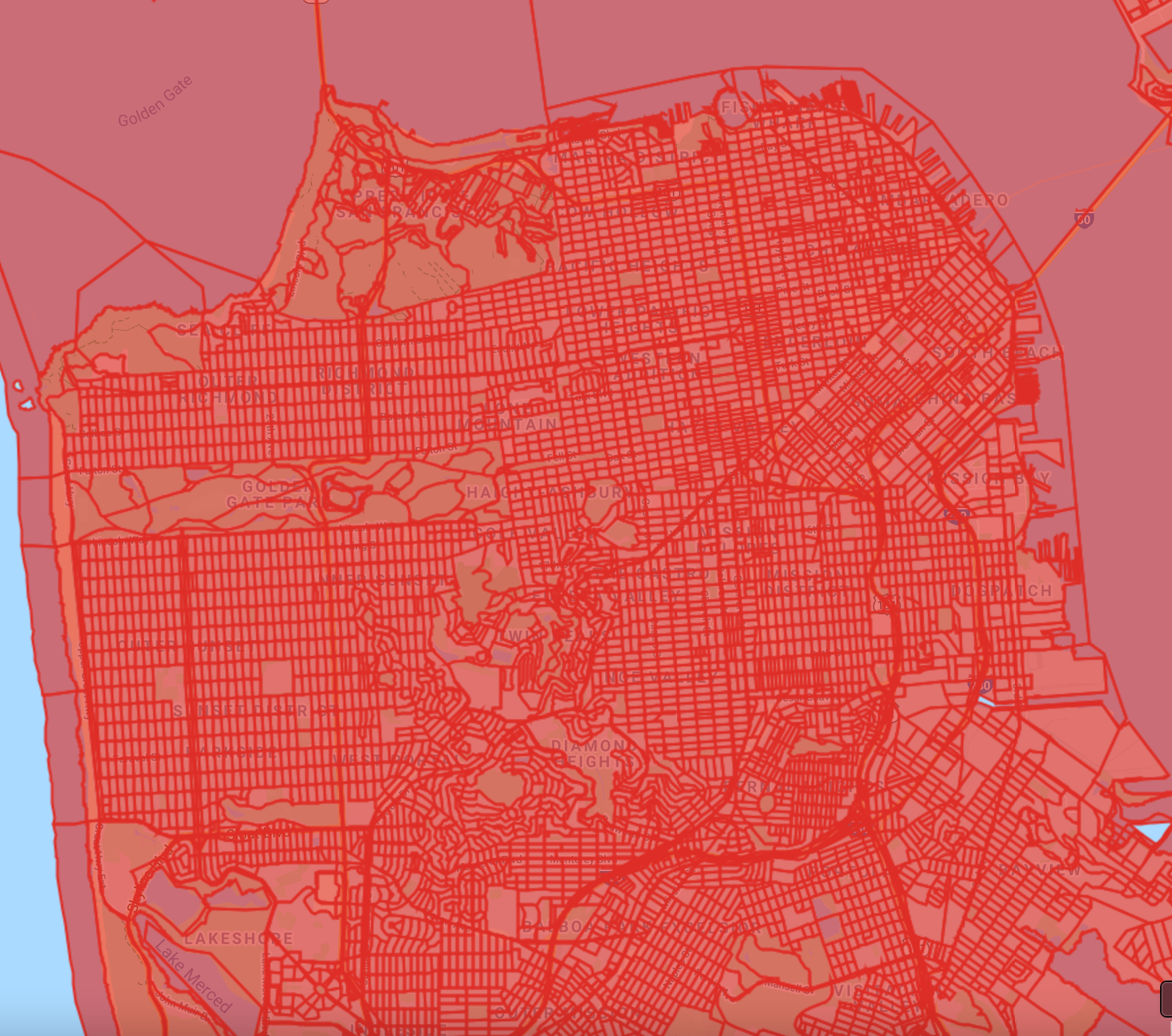
The simplest way to visualize this layer is to use Map.addLayer (Fig. F5.3.1). We can specify a color value in the visParams parameter of the function. Each census block polygon will be rendered with stroke and fill of the specified color. The fill color is the same as the stroke color but has a 66% opacity.

The census blocks table has a property named 'pop10' containing the population totals as of the 2010 census. We can use this to create a choropleth map showing population density. We first need to compute the population density for each feature and add it as a property. To add a new property to each feature, we can map a function over the FeatureCollection and calculate the new property called 'pop_density'. Earth Engine provides the area function, which can calculate the area of a feature in square meters. We convert it to square miles and calculate the population density per square mile.

Now we can use the paint function to create an image from this FeatureCollection using the pop_density property. The paint function needs an empty image that needs to be cast to the appropriate data type. Let’s use the aggregate_stats function to calculate basic statistics for the given column of a FeatureCollection.

You will see that the population density values have a large range. We also have values that are greater than 100,000, so we need to make sure we select a data type that can store values of this size. We create an empty image and cast it to int32, which is able to hold large integer values.

D

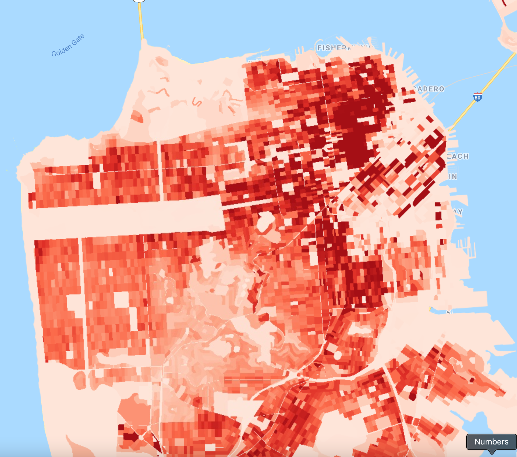
The result is an image with pixel values representing the population density of the polygons. We can now use the standard image visualization method to add this layer to the Map (Fig. F5.3.2). Then, we need to determine minimum and maximum values for the visualization parameters.A reliable technique to produce a good visualization is to find minimum and maximum values that are within one standard deviation. From the statistics that we calculated earlier, we can estimate good minimum and maximum values to be 0 and 50000, respectively.

Section 1.2. Creating a Categorical Map

Continuing the exploration of styling methods, we will now learn about draw and style. These are the preferred methods of styling for points and line layers. Let’s see how we can visualize the TIGER: US Census Roads layer to create a categorical map.

We start by filtering the roads layer to the San Francisco boundary and using Map.addLayer to visualize it.

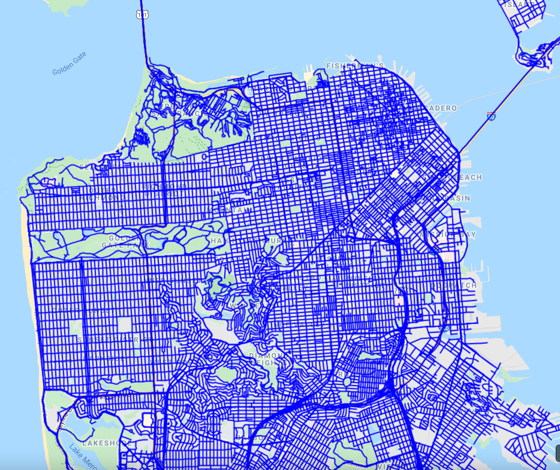
The default visualization renders each line using a width of 2 pixels. The draw function provides a way to specify a different line width. Let’s use it to render the layer with the same color as before but with a line width of 1 pixel (Fig. F5.3.3).

The road layer has a column called “MTFCC” (standing for the MAF/TIGER Feature Class Code). This contains the road priority codes, representing the various types of roads, such as primary and secondary. We can use this information to render each road segment according to its priority. The draw function doesn’t allow us to specify different styles for each feature. Instead, we need to make use of the style function.

The column contains string values indicating different road types as indicated in Table F5.3.1. This full list is available at the MAF/TIGER Feature Class Code Definitions page on the US Census Bureau website.

Table F5.3.1 Census Bureau road priority codes

Let’s say we want to create a map with rules based on the MTFCC values shown in Table F5.3.2.

Table F5.3.2 Styling Parameters for Road Priority Codes

Let’s define a dictionary containing the styling information.

The style function needs a property in the FeatureCollection that contains a dictionary with the style parameters. This allows you to specify a different style for each feature. To create a new property, we map a function over the FeatureCollection and assign an appropriate style dictionary to a new property named 'style'. Note the use of the get function, which allows us to fetch the value for a key in the dictionary. It also takes a default value in case the specified key does not exist. We make use of this to assign different styles to the three road classes specified in Table 5.3.2 and a default style to all others.

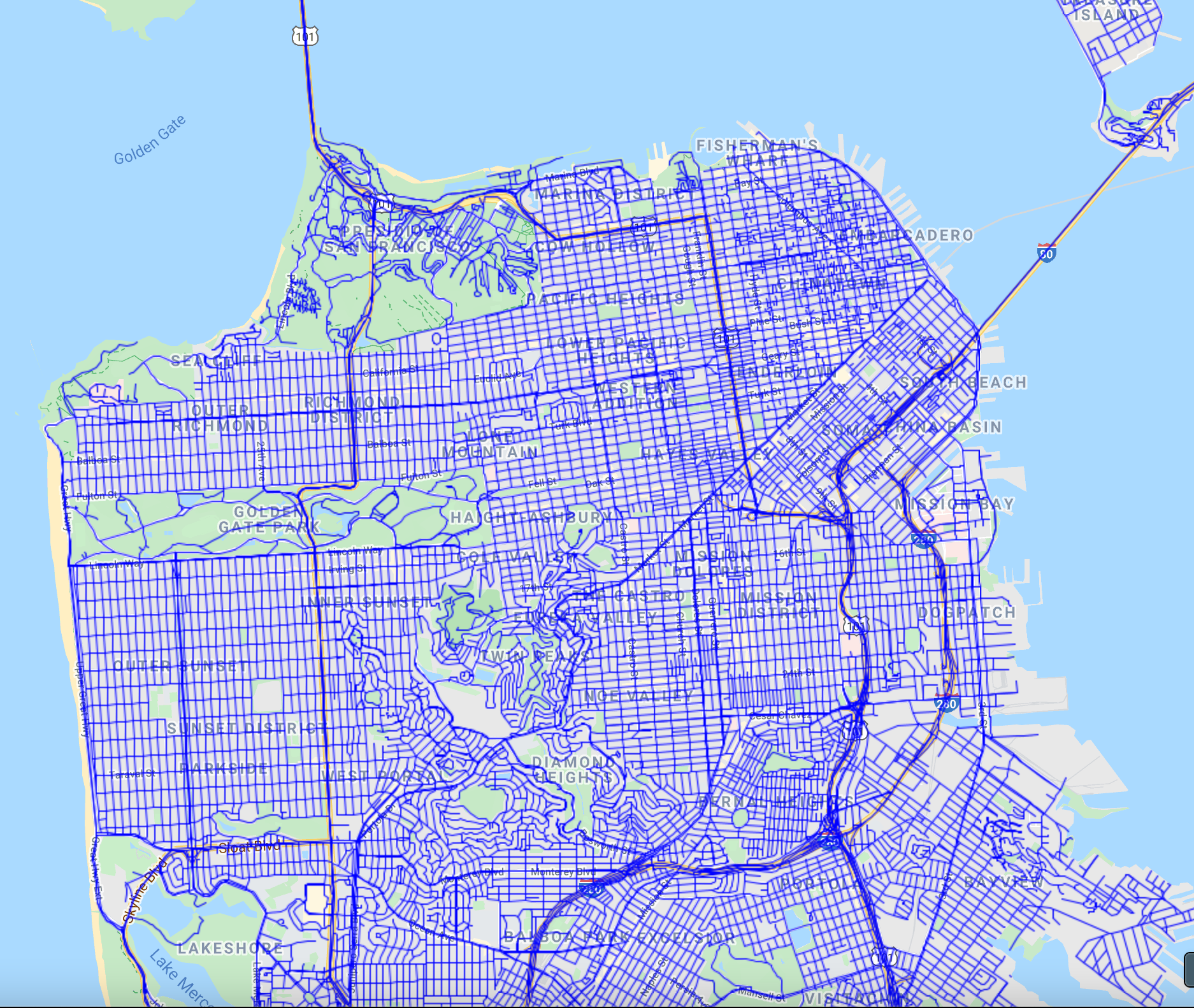
Our collection is now ready to be styled. We call the style function to specify the property that contains the dictionary of style parameters. The output of the style function is an RGB image rendered from the FeatureCollection (Fig. F5.3.4).

Code Checkpoint F53a. The book’s repository contains a script that shows what your code should look like at this point.

Save your script for your own future use, as outlined in Chap. F1.0. Then, refresh the Code Editor to begin with a new script for the next section.

Section 2. Joins with Feature Collections

Earth Engine was designed as a platform for processing raster data, and that is where it shines. Over the years, it has acquired advanced vector data processing capabilities, and users are now able to carry out complex geoprocessing tasks within Earth Engine. You can leverage the distributed processing power of Earth Engine to process large vector layers in parallel.

This section shows how you can do spatial queries and spatial joins using multiple large feature collections. This requires the use of joins. As described for Image Collections in Chap. F4.9, a join allows you to match every item in a collection with items in another collection based on certain conditions. While you can achieve similar results using map and filter, joins perform better and give you more flexibility. We need to define the following items to perform a join on two collections.

1. Filter: A filter defines the condition used to select the features from the two collections. There is a suite of filters in the ee.Filters module that work on two collections, such as ee.Filter.equals and ee.Filter.withinDistance.
2. Join type: While the filter determines which features will be joined, the join type determines how they will be joined. There are many join types, including simple join, inner join, and save-all join.

Joins are one of the harder skills to master, but doing so will help you perform many complex analysis tasks within Earth Engine. We will go through practical examples that will help you understand these concepts and the workflow better.

Section 2.1. Selecting by Location

In this section, we will learn how to select features from one layer that are within a specified distance from features in another layer. We will continue to work with the San Francisco census blocks and roads datasets from the previous section. We will implement a join to select all blocks in San Francisco that are within 1 km of an interstate highway.

We start by loading the census blocks and roads collections and filtering the roads layer to the San Francisco boundary.

As we want to select all blocks within 1 km of an interstate highway, we first filter the sfRoads collection to select all segments with the rttyp property value of I.

We use the draw function to visualize the sfBlocks and interstateRoads layers (Fig. F5.3.5).

Let’s define a join that will select all the features from the sfBlocks layer that are within 1 km of any feature from the interstateRoads layer. We start by defining a filter using the ee.Filter.withinDistance filter. We want to compare the geometries of features in both layers, so we use a special property called '.geo' to compare the collections. By default, the filter will work with exact distances between the geometries. If your analysis does not require a very precise tolerance of spatial uncertainty, specifying a small non-zero maxError distance value will help speed up the spatial operations. A larger tolerance also helps when testing or debugging code so you can get the result quickly instead of waiting longer for a more precise output.

We will use a simple join as we just want features from the first (primary) collection that match the features from the other (secondary) collection.

We can visualize the results in a different color and verify that the join worked as expected (Fig. F5.3.6).

Section 2.2. Spatial Joins

A spatial join allows you to query two collections based on the spatial relationship. We will now implement a spatial join to count points in polygons. We will work with a dataset of tree locations in San Francisco and polygons of neighborhoods to produce a CSV file with the total number of trees in each neighborhood.

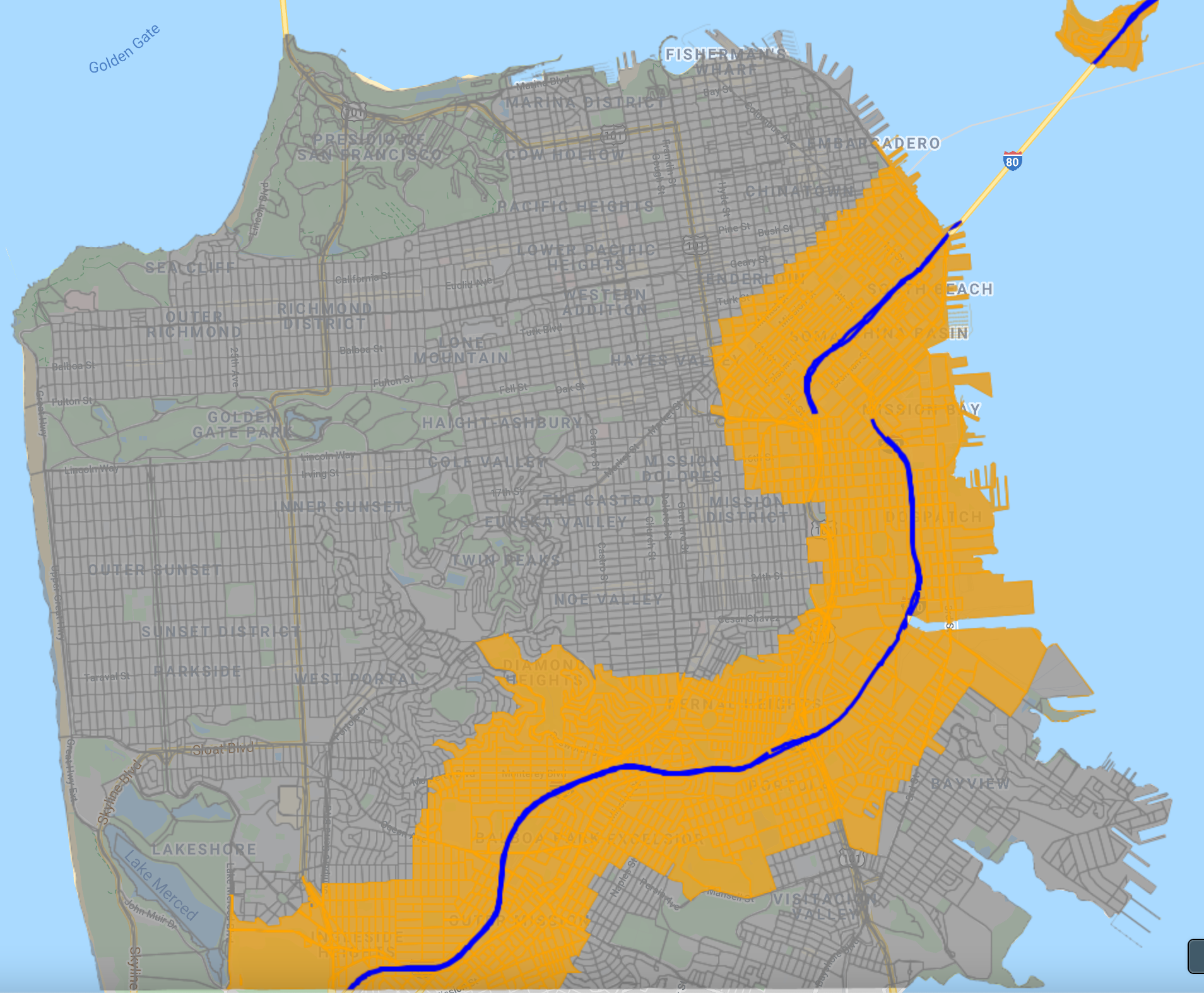
The San Francisco Open Data Portal maintains a street tree map dataset that has a list of street trees with their latitude and longitude. We will also use the San Francisco neighborhood dataset from the same portal. We downloaded, processed, and uploaded these layers as Earth Engine assets for use in this exercise. We start by loading both layers and using the paint and style functions, covered in Sect. 1, to visualize them (Fig. F5.3.7).

To find the tree points in each neighborhood polygon, we will use an ee.Filter.intersects filter.

We need a join that can give us a list of all tree features that intersect each neighborhood polygon, so we need to use a saving join. A saving join will find all the features from the secondary collection that match the filter and store them in a property in the primary collection. Once you apply this join, you will get a version of the primary collection with an additional property that has the matching features from the secondary collection. Here we use the ee.Join.saveAll join, since we want to store all matching features. We specify the matchesKey property that will be added to each feature with the results.

Let’s apply the join and print the first feature of the resulting collection to verify (Fig. F5.3.8).

You will see that each feature of the sfNeighborhoods collection now has an additional property called trees. This contains all the features from the sfTrees collection that were matched using the intersectFilter. We can now map a function over the results and post-process the collection. As our analysis requires the computation of the total number of trees in each neighborhood, we extract the matching features and use the size function to get the count (Fig. F5.3.9).

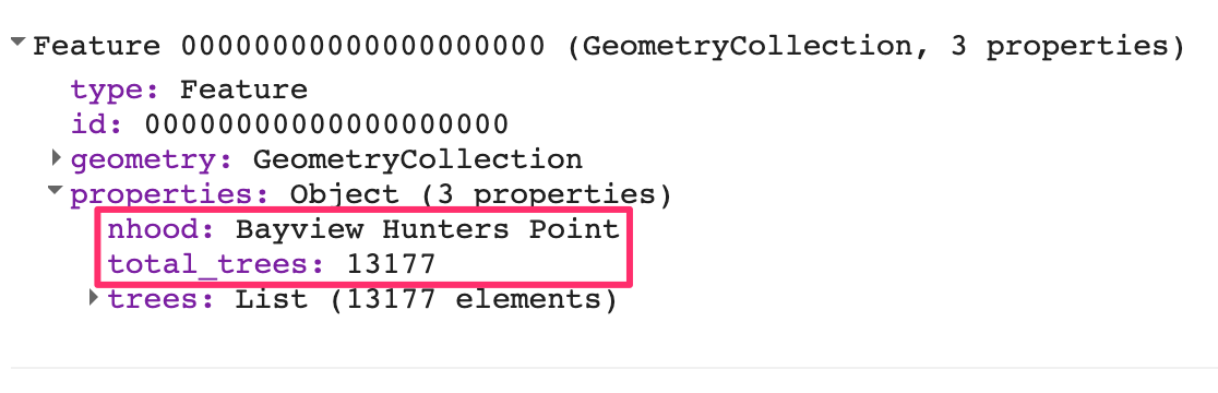
The results now have a property called total_trees containing the count of intersecting trees in each neighborhood polygon.

The final step in the analysis is to export the results as a CSV file using the Export.table.toDrive function. Note that as described in detail in F6.2, you should output only the columns you need to the CSV file. Suppose we do not need all the properties to appear in the output; imagine that wedo not need the trees property, for example, in the output. In that case, we can create only those columns we want in the manner below, by specifying the other selectors parameters with the list of properties to export.

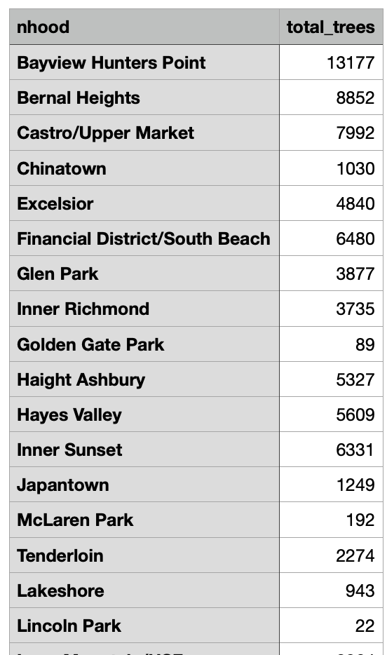
The final result is a CSV file with the neighborhood names and total numbers of trees counted using the join (Fig. F5.3.10).

Code Checkpoint F53b. The book’s repository contains a script that shows what your code should look like at this point.

Synthesis

Assignment 1. What join would you use if you wanted to know which neighborhood each tree belongs to? Modify the code above to do a join and post-process the result to add a neighborhood property to each tree point. Export the results as a shapefile.

Conclusion

This chapter covered visualization and analysis using vector data in Earth Engine. You should now understand different functions for FeatureCollection visualization and be able to create thematic maps with vector layers. You also learned techniques for doing spatial queries and spatial joins within Earth Engine. Earth Engine is capable of handling large feature collections and can be effectively used for many spatial analysis tasks.

Feedback

To review this chapter and make suggestions or note any problems, please go now to bit.ly/EEFA-review. You can find summary statistics from past reviews at bit.ly/EEFA-reviews-stats.

References

Cloud-Based Remote Sensing with Google Earth Engine. (n.d.). CLOUD-BASED REMOTE SENSING WITH GOOGLE EARTH ENGINE. https://www.eefabook.org/

Cloud-Based Remote Sensing with Google Earth Engine. (2024). In Springer eBooks. https://doi.org/10.1007/978-3-031-26588-4