Aquatic and Hydrological Applications

Benthic Habitats

Cloud-Based Remote Sensing with Google Earth Engine

Fundamentals and Applications

Part A2: Aquatic and Hydrological Applications

Earth Engine’s global scope and long time series allow analysts to understand the water cycle in new and unique ways. These include surface water in the form of floods and river characteristics, long-term issues of water balance, and the detection of subsurface ground water.

Chapter A2.2: Benthic Habitats

Authors:

Dimitris Poursanidis, Aurélie C. Shapiro, Spyros Christofilakos

Overview

Shallow-water coastal benthic habitats, which can comprise seagrasses, sandy soft bottoms, and coral reefs, are essential ecosystems, supporting fisheries, providing coastal protection, and sequestering “blue” carbon. Multispectral satellite imagery, particularly with blue and green spectral bands, can penetrate clear, shallow water, allowing us to identify what lies on the seafloor. In terrestrial habitats, atmospheric and topographic corrections are important, whereas in shallow waters, it is essential to correct the effects of the water column, as different depths can change the reflectance observed by the satellite sensor. Once you know water depth, you can accurately assess benthic habitats such as seagrass, sand, and coral. In this chapter, we will describe how to estimate water depth from high-resolution Planet data and map benthic habitats.

Learning Outcomes

Separating land from water with a supervised classification.
Identifying and classifying benthic habitats using machine learning.
Removing surface sunglint and wave glint.
Developing regression models to estimate water depth using training data.
Correcting for water depth to derive bottom surface reflectance through a regression approach.
Evaluating training data and model accuracy.

Helps if you know how to:

Import images and image collections, filter, and visualize (Part F1).
Perform basic image analysis: select bands, compute indices, create masks, classify images (Part F2).
Use normalizedDifference to calculate vegetation indices (Chap. F2.0).
Use drawing tools to create points, lines, and polygons (Chap. F2.1).
Perform a supervised Random Forest image classification (Chap. F2.1).
Obtain accuracy metrics from classifications (Chap. F2.2).
Use reducers to implement linear regression between image bands (Chap. F3.0).
Filter a FeatureCollection to obtain a subset (Chap. F5.0, Chap. F5.1).
Convert between raster and vector data (Chap. F5.1).

Github Code link for all tutorials

This code base is collection of codes that are freely available from different authors for google earth engine.

Github Source

Introduction to Theory

Coastal benthic habitats include several ecosystems across the globe. One common element is the seagrass meadow, a significant component of coastal marine ecosystems (UNEP/MAP 2012). Seagrass meadows are among the most productive habitats in the coastal zone, performing essential ecosystem functions and providing essential ecosystem services (Duarte et al. 2011), such as water oxygenation and nutrient provision, seafloor and beach stabilization (as sediment is controlled and trapped within the rhizomes of the meadows), carbon burial, and nursery areas and refuge for commercial and endemic species (Boudouresque et al. 2012, Vassallo et al. 2013, Campagne et al. 2015).

However, seagrass meadows are experiencing a global decline due to intensive human activities and climate change (Boudouresque et al. 2009). Threats from climate change include sea surface temperature increases and sea level rise, as well as more frequent and intensive storms (Pergent 2014). These threats represent a pressing challenge for coastal management and are predicted to have deleterious effects on seagrasses.

Several programs have focused on coastal seabed mapping, and a wide range of methods have been utilized for mapping seagrasses (Borfecchia et al. 2013, Eugenio et al. 2015). Satellite remote sensing has been employed for the mapping of seagrass meadows and coral reefs in several areas (Goodman et al. 2013, Hedley et al. 2016, Knudby and Nordlund 2011, Koedsin et al. 2016, Lyons et al. 2012).

In this chapter, we will show you how to map coastal habitats using high-resolution Earth observation data from Planet with updated field data collected in the same period as the imagery acquisition. You will learn how to calculate coastal bathymetry using high-quality field data and machine learning regression methods. In the end, you will be able to adapt the code and use your own data to work in your own coastal area of interest, which can be tropical or temperate as long as there are clear waters up to 30 m deep.

Practicum

Section 1. Inputting Data

The first step is to define the data that you will work on. By uploading raster and vector data via the Earth Engine asset inventory, you will be able to analyze and process them through the Earth Engine API. The majority of satellite data are stored with values scaled by 10000 and truncated in order to occupy less memory. In this setting, it is crucial to scale them back to their physical values before processing them.

// Section 1
// Import and display satellite image.
var planet=ee.Image('projects/gee-book/assets/A2-2/20200505_N2000')
.divide(10000);

Map.centerObject(planet, 12);
var visParams={
bands: ['b3', 'b2', 'b1'],
min: 0.17,
max: 0.68,
gamma: 0.8
};
Map.addLayer({
eeObject: planet,
visParams: visParams,
name: 'planet initial',
shown: true
});

Code Checkpoint A22a. The book’s repository contains a script that shows what your code should look like at this point.

Section 2. Preprocessing Functions

Code Checkpoint A22b. The book’s repository contains a script to use to begin this section. You will need to start with that script and paste code below into it. When you run the script, you will see several assets being imported for water, land, sunglint and sandy patches to correct for the water column.

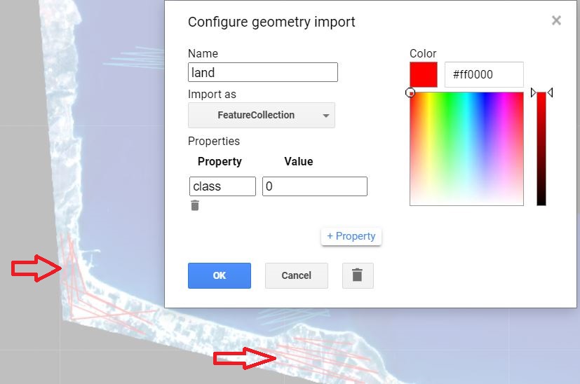
With the Planet imagery imported into Earth Engine, we now need to prepare for the classification and bathymetry procedures that will follow. The aim of the preprocessing is to correct or minimize spectral alterations due to physical conditions like sunglint, waves, and the water column. The landmask function below will remove the land area from our image in order to focus on the marine area of interest. This prevents the land reflectance values, which are relatively high, from biasing the main process of detection over relatively dark water. To implement this step, we will perform a supervised classification to obtain the land/water mask. To prepare for the classification, we drew water and land geometry imports and set them as a FeatureCollection with property 'class' and values 1 and 0, respectively (Fig. A2.2.1). We will employ the Normalized Difference Water Index (NDWI) (Gao 1996) using a Random Forest classifier (Breiman 2001). Due to the distinct spectral reflectances of terrain and water surfaces, there is no need to ensure a balanced dataset between the two classes. However, the size of the training dataset is still important and therefore, the more the better. For this task, we create ‘line’ geometries because we can get more training points than ‘point’ geometries with fewer clicks. For more information regarding generating training lines, points or polygons, please see Chap. F2.1.

Fig. A2.2.1 Labeling of land and water regions using lines in preparation for the Random Forests classification

// Section 2
// Mask based to NDWI and RF.
function landmask(img){
var ndwi=img.normalizedDifference(['b2', 'b4']);
var training=ndwi.sampleRegions(land.merge(water), ['class'],
3);
var trained=ee.Classifier.smileRandomForest(10)
.train(training, 'class');
var classified=ndwi.classify(trained);
var mask=classified.eq(1);

return img.updateMask(mask);
}

var maskedImg=landmask(planet);

Map.addLayer(maskedImg, visParams, 'maskedImg', false);

Sunglint is a phenomenon that occurs when the sun angle and the sensor are positioned such that there is a mirror-like reflection at the water surface. In areas of glint, we cannot detect reflectance from the ocean floor. This will affect image processing and needs to be corrected. The user adds polygons identifying areas of glint (Fig. A2.2.2), and these areas are removed using linear modeling (Hedley et al. 2005).

// Sun-glint correction.
function sunglintRemoval(img){
var linearFit1=img.select(['b4', 'b1']).reduceRegion({
reducer: ee.Reducer.linearFit(),
geometry: sunglint,
scale: 3,
maxPixels: 1e12,
bestEffort: true,
});
var linearFit2=img.select(['b4', 'b2']).reduceRegion({
reducer: ee.Reducer.linearFit(),
geometry: sunglint,
scale: 3,
maxPixels: 1e12,
bestEffort: true,
});
var linearFit3=img.select(['b4', 'b3']).reduceRegion({
reducer: ee.Reducer.linearFit(),
geometry: sunglint,
scale: 3,
maxPixels: 1e12,
bestEffort: true,
});

var slopeImage=ee.Dictionary({
'b1': linearFit1.get('scale'),
'b2': linearFit2.get('scale'),
'b3': linearFit3.get('scale')
}).toImage();

var minNIR=img.select('b4').reduceRegion({
reducer: ee.Reducer.min(),
geometry: sunglint,
scale: 3,
maxPixels: 1e12,
bestEffort: true,
}).toImage(['b4']);

return img.select(['b1', 'b2', 'b3'])
.subtract(slopeImage.multiply((img.select('b4')).subtract(
minNIR)))
.addBands(img.select('b4'));
}
var sgImg=sunglintRemoval(maskedImg);
Map.addLayer(sgImg, visParams, 'sgImg', false);

Fig. A2.2.2 Identification of areas with sunglint. Raising the gamma parameter during the visualization makes the phenomenon appear more intense, making it easier to draw the glint polygons.

Question 1. If you design more polygons fοr sunglint correction, can you see any improvement in the results visually and by examining values in pixels? Keep in mind that in already drawn rectangles (sunglint polygons), you can not draw free shaped polygons or lines. Try instead adding some more points or rectangles

You can design more polygons, or select areas with severe or moderate sunglint to see how the site selection influences the final results.

The Depth Invariant Index (DIV) is a tool that creates a proxy image that helps minimize the bias of the spectral values due to the water column during classification and bathymetry procedures. Spectral signatures tend to be affected by the depth of the water column due to suspended material and the absorption of light. A typical result is that shallow seagrasses and deeper sandy seafloors will have similar spectral signatures. The correction of that error is based on the correlation between depth and logged bands (Lyzenga 1981).

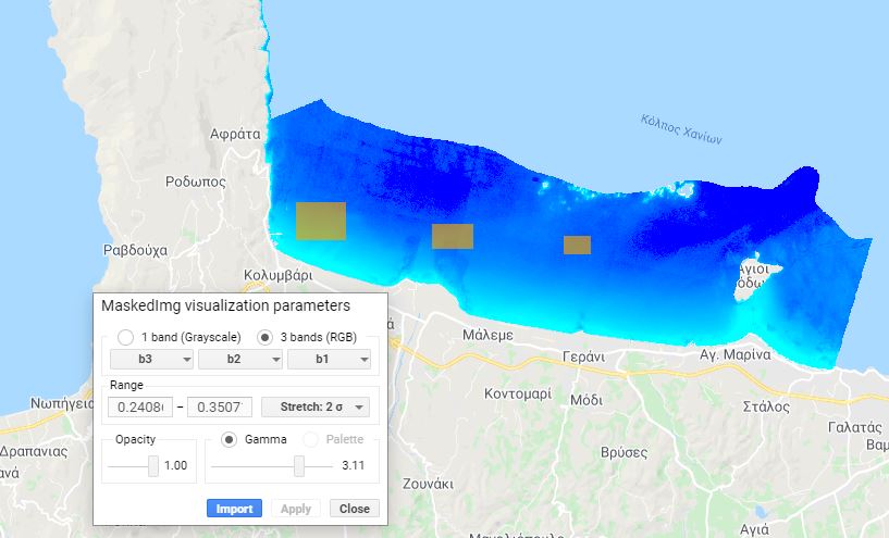
In our example, the correction of water column alterations is based on the ratio of the green and blue bands, because of their higher penetrating properties compared to the red and near-infrared (NIR) bands. As in the previous functions, a requirement for this procedure is to identify sandy patches in different depth ranges. If needed, you can use the satellite layer to do so.

Since we will use log values in the current step, it is crucial to transform all the negative values to positive before estimating DIV. Therefore, and since the majority of the values are in optically deep waters, the value 0.0001 will be assigned to values less than 0 in an attempt to avoid altering the pixels with positive values at the coastal zone. Moreover, a low-pass filter will be applied to normalize the observed noise that occurred during the previous steps (see Sect. F3.2).

// DIV procedure.
function kernel(img){
var boxcar=ee.Kernel.square({
radius: 2,
units: 'pixels',
normalize: true
});
return img.convolve(boxcar);
}

function makePositive(img){
return img.where(img.lte(0), 0.0001);
}

function div(img){
var band1=ee.List(['b1', 'b2', 'b3', 'b1', 'b2']);
var band2=ee.List(['b3', 'b3', 'b2', 'b2', 'b1']);
var nband=ee.List(['b1b3', 'b2b3', 'b3b2', 'b1b2', 'b2b1']);

for (var i=0; i < 5; i +=1) {
var x=band1.get(i);
var y=band2.get(i);
var z=nband.get(i);

var imageLog=img.select([x, y]).log();

var covariance=imageLog.toArray().reduceRegion({
reducer: ee.Reducer.covariance(),
geometry: DIVsand,
scale: 3,
maxPixels: 1e12,
bestEffort: true,
});

var covarMatrix=ee.Array(covariance.get('array'));
var var1=covarMatrix.get([0, 0]);
var var2=covarMatrix.get([1, 1]);
var covar=covarMatrix.get([0, 1]);

var a=var1.subtract(var2).divide(covar.multiply(2));
var attenCoeffRatio=a.add(((a.pow(2)).add(1)).sqrt());

var depthInvariantIndex=img.expression(
'image1 - (image2 * coeff)', {
'image1': imageLog.select([x]),
'image2': imageLog.select([y]),
'coeff': attenCoeffRatio
});

img=ee.Image.cat([img, depthInvariantIndex.select([x], [
z
])]);
}
return img;
}

var divImg=div(kernel(makePositive(sgImg))).select('b[1-3]',
'b1b2');
var vivVisParams={
bands: ['b1b2'],
min: -0.81,
max: -0.04,
gamma: 0.75
};
Map.addLayer(divImg, vivVisParams, 'divImg', false);

Question 2. How can the selection of sandy patches influence the final result?

Sandy patches can also include signals from sparse seagrass or other types of benthic cover. Select different areas of variable depths and therefore different spectral reflectance to explore the changes in the final DIV result.

Code Checkpoint A22c. The book’s repository contains a script that shows what your code should look like at this point.

Section 3. Supervised Classification

To create accurate classifications, it is beneficial for the training data set to be created from in situ data. This is especially important in marine remote sensing, due to dynamic, varying ecosystems. In our example, all the reference data were acquired during scientific dives. The reference data consist of three classes: SoftBottom for Sandy patches, rockyBottom for rocky patches and pO for posidonia-seagrass patches. Here, we provide a dataset that will be split using a 70%-30% partitioning strategy into training and validation data (see Sect. F2.1) and is already pre-loaded in the assets of this book.

// Section 3, classification
// Import of reference data and split.
var softBottom=ee.FeatureCollection(
'projects/gee-book/assets/A2-2/SoftBottom');
var rockyBottom=ee.FeatureCollection(
'projects/gee-book/assets/A2-2/RockyBottom');
var pO=ee.FeatureCollection('projects/gee-book/assets/A2-2/PO');

var sand=ee.FeatureCollection.randomPoints(softBottom, 150).map(
function(s){
return s.set('class', 0);
}).randomColumn();
var sandT=sand.filter(ee.Filter.lte('random', 0.7)).aside(print,
'sand training');
var sandV=sand.filter(ee.Filter.gt('random', 0.7)).aside(print,
'sand validation');
Map.addLayer(sandT,{
color: 'yellow'
}, 'Sand Training', false);
Map.addLayer(sandV,{
color: 'yellow'
}, 'Sand Validation', false);

var hard=ee.FeatureCollection.randomPoints(rockyBottom, 79).map(
function(s){
return s.set('class', 1);
}).randomColumn();
var hardT=hard.filter(ee.Filter.lte('random', 0.7)).aside(print,
'hard training');
var hardV=hard.filter(ee.Filter.gt('random', 0.7)).aside(print,
'hard validation');
Map.addLayer(hardT,{
color: 'red'
}, 'Rock Training', false);
Map.addLayer(hardV,{
color: 'red'
}, 'Rock Validation', false);

var posi=pO.map(function(s){
return s.set('class', 2);
})
.randomColumn('random');
var posiT=posi.filter(ee.Filter.lte('random', 0.7)).aside(print,
'posi training');
var posiV=posi.filter(ee.Filter.gt('random', 0.7)).aside(print,
'posi validation');
Map.addLayer(posiT,{
color: 'green'
}, 'Posidonia Training', false);
Map.addLayer(posiV,{
color: 'green'
}, 'Posidonia Validation', false);

For this procedure, we chose the ee.Classifier.libsvm classifier because of its established performance in aquatic environments (Poursanidis et al. 2018, da Silveira et al. 2021). The function below does the classification and also estimates overall, user’s, and producer’s accuracy (see Chap. F2.2):

// Classification procedure.
function classify(img){
var mergedT=ee.FeatureCollection([sandT, hardT, posiT])
.flatten();
var training=img.sampleRegions(mergedT, ['class'], 3);
var trained=ee.Classifier.libsvm({
kernelType: 'RBF',
gamma: 1,
cost: 500
}).train(training, 'class');
var classified=img.classify(trained);

var mergedV=ee.FeatureCollection([sandV, hardV, posiV])
.flatten();
var accuracyCol=classified.unmask().reduceRegions({
collection: mergedV,
reducer: ee.Reducer.first(),
scale: 10
});
var classificationErrorMatrix=accuracyCol.errorMatrix({
actual: 'class',
predicted: 'first',
order: [0, 1, 2]
});
var classNames=['soft_bot', 'hard_bot', 'seagrass'];
var accuracyOA=classificationErrorMatrix.accuracy();
var accuraccyCons=ee.Dictionary.fromLists({
keys: classNames,
values: classificationErrorMatrix.consumersAccuracy()
.toList()
.flatten()
});
var accuracyProd=ee.Dictionary.fromLists({
keys: classNames,
values: classificationErrorMatrix.producersAccuracy()
.toList()
.flatten()
});

var classificationErrormatrixArray=classificationErrorMatrix
.array();

var arrayToDatatable=function(array){
var classesNames=ee.List(classNames);

function toTableColumns(s){
return {
id: s,
label: s,
type: 'number'
};
}
var columns=classesNames.map(toTableColumns);

function featureToTableRow(f){
return {
c: ee.List(f).map(function(c){
return {
v: c
};
})
};
}
var rows=array.toList().map(featureToTableRow);
return ee.Dictionary({
cols: columns,
rows: rows
});
};

var dataTable=arrayToDatatable(classificationErrormatrixArray)
.evaluate(function(dataTable){
print('------------- Error matrix -------------',
ui.Chart(dataTable, 'Table')
.setOptions({
pageSize: 15
}),
'rows: reference, cols: mapped');
});
print('Overall Accuracy', accuracyOA);
print('Users accuracy', accuraccyCons);
print('Producers accuracy', accuracyProd);
return classified;
}

var svmClassification=classify(divImg);
var svmVis={
min: 0,
max: 2,
palette: ['ffffbf', 'fc8d59', '91cf60']
};
Map.addLayer(svmClassification, svmVis, 'classification');

Code Checkpoint A22d. The book’s repository contains a script that shows what your code should look like at this point.

Section 4. Bathymetry by Random Forests regression

For the bathymetry procedure, we will exploit the setOutputMode('REGRESSION') option of ee.Classifier.smileRandomForest. For this example, reference data came from a sonar that was mounted on a boat. In contrast to the classification accuracy assessment, the accuracy assessment of bathymetry is based on and the root-mean-square error (RMSE).

With regard to visualization of the resulting bathymetry, we have to consider the selection of colors and their physical meanings. In the classification, which is a categorical image, we use a diverging palette, while in bathymetry, which shows a continuous value, we should use a sequential palette. Tip: “cold” colors better convey depth. For the satellite derived bathymetry we use preloaded assets with the in-situ depth measurement. The quality of these measurements is crucial to the success of the classifier.

// Section 4, Bathymetry
// Import and split training and validation data for the bathymetry.
var depth=ee.FeatureCollection(
'projects/gee-book/assets/A2-2/DepthDataTill09072020_v2');
depth=depth.randomColumn();
var depthT=depth.filter(ee.Filter.lte('random', 0.7));
var depthV=depth.filter(ee.Filter.gt('random', 0.7));
Map.addLayer(depthT,{
color: 'black'
}, 'Depth Training', false);
Map.addLayer(depthV,{
color: 'gray'
}, 'Depth Validation', false);

So that every pixel contains at most one measurement, the vector depth assets are rasterized prior to using them for the regression.

Finally, we need to write down and execute the function to calculate the satellite derived bathymetry function, based on the Random Forest classifier.

Question 3. Does the selection of different color ramps lead to misinterpretations?

By choosing different color ramps for the same data set, you can see how visual interpretation can be changed based on color. Trying different color ramps will reveal how some can better visualize the final results for further use in maritime spatial planning activities, while others, including commonly seen rainbow ramps, can lead to erroneous decisions.

Code Checkpoint A22e. The book’s repository contains a script that shows what your code should look like at this point.

Synthesis

With what you learned in this chapter, you can analyze Earth observation data—here, specifically from the Planet Cubesat constellation—to create your own map of coastal benthic habitats and coastal bathymetry for a specific case study. Feel free to test out the approach in another part of the world using your own data or open-access data, or use your own training data for a more refined classification model.

You can add your own point data to the map, collected via a fieldwork campaign or by visually interpreting the imagery, and merge with the training data to improve a classification, or clean areas that need to be removed by drawing polygons and masking them in the classification.

For the bathymetry, you can select different calibration/validation ratio approaches and test the optimum ratio of splitting to see how it influences the final bathymetry map. You can also add a smoothing filter to create a visually smoother image of coastal bathymetry.

Conclusion

Many coastal habitats, especially seagrass meadows, are dynamic ecosystems that change over time and can be lost through natural and anthropogenic causes.

The power of Earth Engine lies in its cloud-based, lightning-fast, automated approach to workflows, especially its automated training data collection and processing power. This process would take days when performed offline in traditional remote-sensing software, especially over large areas. And the Earth Engine approach is not only fast but also consistent: The same method can be applied to images from different dates to assess habitat changes over time, both gain and loss.

The availability of Planet imagery allows us to use a high-resolution product. Natively, Earth Engine hosts the archives of Sentinel-2 and Landsat data. The Landsat archive spans from 1984 to the present, while Sentinel-2, a higher-resolution product, is available from 2017 to today. All of this imagery can be used in the same workflow in order to map benthic habitats and monitor their changes over time, allowing us to understand the past of the coastal seascape and envision its future.

Feedback

To review this chapter and make suggestions or note any problems, please go now to bit.ly/EEFA-review. You can find summary statistics from past reviews at bit.ly/EEFA-reviews-stats.

References

Cloud-Based Remote Sensing with Google Earth Engine. (n.d.). CLOUD-BASED REMOTE SENSING WITH GOOGLE EARTH ENGINE. https://www.eefabook.org/

Cloud-Based Remote Sensing with Google Earth Engine. (2024). In Springer eBooks. https://doi.org/10.1007/978-3-031-26588-4

Borfecchia F, Micheli C, Carli F, et al (2013) Mapping spatial patterns of Posidonia oceanica meadows by means of Daedalus ATM airborne sensor in the coastal area of Civitavecchia (Central Tyrrhenian Sea, Italy). Remote Sens 5:4877–4899. https://doi.org/10.3390/rs5104877

Boudouresque CF, Bernard G, Pergent G, et al (2009) Regression of Mediterranean seagrasses caused by natural processes and anthropogenic disturbances and stress: A critical review. Bot Mar 52:395–418. https://doi.org/10.1515/BOT.2009.057

Boudouresque CF, Bernard G, Bonhomme P, et al (2012) Protection and Conservation of Posidonia oceanica Meadows. RAMOGE and RAC/SPA

Breiman L (2001) Random forests. Mach Learn 45:5–32. https://doi.org/10.1023/A:1010933404324

Campagne CS, Salles JM, Boissery P, Deter J (2014) The seagrass Posidonia oceanica: Ecosystem services identification and economic evaluation of goods and benefits. Mar Pollut Bull 97:391–400. https://doi.org/10.1016/j.marpolbul.2015.05.061

da Silveira CBL, Strenzel GMR, Maida M, et al (2021) Coral reef mapping with remote sensing and machine learning: A nurture and nature analysis in marine protected areas. Remote Sens 13:2907. https://doi.org/10.3390/rs13152907

Duarte CM, Kennedy H, Marbà N, Hendriks I (2013) Assessing the capacity of seagrass meadows for carbon burial: Current limitations and future strategies. Ocean Coast Manag 83:32–38. https://doi.org/10.1016/j.ocecoaman.2011.09.001

Eugenio F, Marcello J, Martin J (2015) High-resolution maps of bathymetry and benthic habitats in shallow-water environments using multispectral remote sensing imagery. IEEE Trans Geosci Remote Sens 53:3539–3549. https://doi.org/10.1109/TGRS.2014.2377300

Gao BC (1996) NDWI - A normalized difference water index for remote sensing of vegetation liquid water from space. Remote Sens Environ 58:257–266. https://doi.org/10.1016/S0034-4257(96)00067-3

Goodman J, Purkis S, Phinn SR (2011) Coral Reef Remote Sensing: A Guide for Mapping, Monitoring and Management. Springer

Hedley JD, Harborne AR, Mumby PJ (2005) Simple and robust removal of sun glint for mapping shallow-water benthos. Int J Remote Sens 26:2107–2112. https://doi.org/10.1080/01431160500034086

Hedley JD, Roelfsema CM, Chollett I, et al (2016) Remote sensing of coral reefs for monitoring and management: A review. Remote Sens 8:118. https://doi.org/10.3390/rs8020118

Knudby A, Nordlund L (2011) Remote sensing of seagrasses in a patchy multi-species environment. Int J Remote Sens 32:2227–2244. https://doi.org/10.1080/01431161003692057

Koedsin W, Intararuang W, Ritchie RJ, Huete A (2016) An integrated field and remote sensing method for mapping seagrass species, cover, and biomass in Southern Thailand. Remote Sens 8:292. https://doi.org/10.3390/rs8040292

Lyzenga DR (1981) Remote sensing of bottom reflectance and water attenuation parameters in shallow water using aircraft and Landsat data. Int J Remote Sens 2:71–82. https://doi.org/10.1080/01431168108948342

Pergent G, Bazairi H, Bianchi CN, et al (2014) Climate change and Mediterranean seagrass meadows: A synopsis for environmental managers. Mediterr Mar Sci 15:462–473. https://doi.org/10.12681/mms.621

Poursanidis D, Topouzelis K, Chrysoulakis N (2018) Mapping coastal marine habitats and delineating the deep limits of the Neptune’s seagrass meadows using very high resolution Earth observation data. Int J Remote Sens 39:8670–8687. https://doi.org/10.1080/01431161.2018.1490974

UNEP/MAP (2009) State of the Mediterranean marine and coastal environment. In: Ecological Applications. pp 1047–1056