Cloud-Based Remote Sensing with Google Earth Engine
Fundamentals and Applications

Part F5: Vectors and Tables
In addition to raster data processing, Earth Engine supports a rich set of vector processing tools. This Part introduces you to the vector framework in Earth Engine, shows you how to create and to import your vector data, and how to combine vector and raster data for analyses.
Chapter F5.2: Zonal Statistics
Authors
Sara Winsemius and Justin Braaten
Overview
The purpose of this chapter is to extract values from rasters for intersecting points or polygons. We will lay out the process and a function to calculate zonal statistics, which includes optional parameters to modify the function, and then apply the process to three examples using different raster datasets and combinations of parameters.
Learning Outcomes
- Buffering points as square or circular regions.
- Writing and applying functions with optional parameters.
- Learning what zonal statistics are and how to use reducers.
- Exporting computation results to a table.
- Copying properties from one image to another.
Assumes you know how to:
- Recognize similarities and differences among Landsat 5, 7, and 8 spectral bands (Part F1, Part F2, Part F3).
- Understand distinctions among Image, ImageCollection, Feature and FeatureCollection Earth Engine objects (Part F1, Part F2, Part F5).
- Use drawing tools to create points, lines, and polygons (Chap. F2.1).
- Write a function and map it over an ImageCollection (Chap. F4.0).
- Mask cloud, cloud shadow, snow/ice, and other undesired pixels (Chap. F4.3).
- Export calculated data to tables with Tasks (Chap. F5.0).
- Understand the differences between raster and vector data (Chap. F5.0, Chap. F5.1).
- Write a function and map it over a FeatureCollection (Chap. F5.1).
Github Code link for all tutorials
This code base is collection of codes that are freely available from different authors for google earth engine.
Introduction to Theory
Anyone working with field data collected at plots will likely need to summarize raster-based data associated with those plots. For instance, they need to know the Normalized Difference Vegetation Index (NDVI), precipitation, or elevation for each plot (or surrounding region). Calculating statistics from a raster within given regions is called zonal statistics. Zonal statistics were calculated in Chaps. F5.0 and F5.1 using ee.Image.ReduceRegions. Here, we present a more general approach to calculating zonal statistics with a custom function that works for both ee.Image and ee.ImageCollection objects. In addition to its flexibility, the reduction method used here is less prone to “Computed value is too large” errors that can occur when using ReduceRegions with very large or complex ee.FeatureCollection object inputs.
The zonal statistics function in this chapter works for an Image or an ImageCollection. Running the function over an ImageCollection will produce a table with values from each image in the collection per point. Image collections can be processed before extraction as needed—for example, by masking clouds from satellite imagery or by constraining the dates needed for a particular research question. In this tutorial, the data extracted from rasters are exported to a table for analysis, where each row of the table corresponds to a unique point-image combination.
In fieldwork, researchers often work with plots, which are commonly recorded as polygon files or as a center point with a set radius. It is rare that plots will be set directly in the center of pixels from your desired raster dataset, and many field GPS units have positioning errors. Because of these issues, it may be important to use a statistic of adjacent pixels (as described in Chap. F3.2) to estimate the central value in what’s often called a neighborhood mean or focal mean (Cansler and McKenzie 2012, Miller and Thode 2007).
To choose the size of your neighborhood, you will need to consider your research questions, the spatial resolution of the dataset, the size of your field plot, and the error from your GPS. For example, the raster value extracted for randomly placed 20 m diameter plots would likely merit use of a neighborhood mean when using Sentinel-2 or Landsat 8—at 10 m and 30 m spatial resolution, respectively—while using a thermal band from MODIS (Moderate Resolution Imaging Spectroradiometer) at 1000 m may not. While much of this tutorial is written with plot points and buffers in mind, a polygon asset with predefined regions will serve the same purpose.
Practicum
Section 1. Functions
Two functions are provided; copy and paste them into your script:
- A function to generate circular or square regions from buffered points
- A function to extract image pixel neighborhood statistics for a given region
Section 1.1. Function: bufferPoints(radius, bounds)
Our first function, bufferPoints, returns a function for adding a buffer to points and optionally transforming to rectangular bounds (see Table F5.2.1).
Table F5.2.1 Parameters for bufferPoints
Parameter | Type | Description |
radius | Number | buffer radius (m). |
[bounds=false] | Boolean | An optional flag indicating whether to transform buffered point (i.e., a circle) to square bounds. |
function bufferPoints(radius, bounds) { |
Section 1.2. Function: zonalStats(fc, params)
The second function, zonalStats, reduces images in an ImageCollection by regions defined in a FeatureCollection. Note that reductions can return null statistics that you might want to filter out of the resulting feature collection. Null statistics occur when there are no valid pixels intersecting the region being reduced. This situation can be caused by points that are outside of an image or in regions that are masked for quality or clouds.
This function is written to include many optional parameters (see Table F5.2.2). Look at the function carefully and note how it is written to include defaults that make it easy to apply the basic function while allowing customization.
Table F5.2.2 Parameters for zonalStats
Parameter | Type | Description |
ic | ee.ImageCollection | Image collection from which to extract values. |
fc | ee.FeatureCollection | Feature collection that provides regions/zones by which to reduce image pixels. |
[params] | Object | An optional Object that provides function arguments. |
[params.reducer=ee.Reducer.mean()] | ee.Reducer | The reducer to apply. Optional. |
[params.scale=null] | Number | A nominal scale in meters of the projection to work in. If null, the native nominal image scale is used. Optional. |
[params.crs=null] | String | The projection to work in. If null, the native image Coordinate Reference System (CRS) is used. Optional. |
[params.bands=null] | Array | A list of image band names for which to reduce values. If null, all bands will be reduced. Band names define column names in the resulting reduction table. Optional. |
[params.bandsRename=null] | Array | A list of desired image band names. The length and order must correspond to the params.bands list. If null, band names will be unchanged. Band names define column names in the resulting reduction table. Optional. |
[params.imgProps=null] | Array | A list of image properties to include in the table of region reduction results. If null, all image properties are included. Optional. |
[params.imgPropsRename=null] | Array | A list of image property names to replace those provided by params.imgProps. The length and order must match the params.imgProps entries. Optional. |
[params.datetimeName='datetime] | String | The desired name of the datetime field. The datetime refers to the 'system:time_start' value of the ee.Image being reduced. Optional. |
[params.datetimeFormat='YYYY-MM-dd HH:mm:ss] | String | The desired datetime format. Use ISO 8601 data string standards. The datetime string is derived from the 'system:time_start' value of the ee.Image being reduced. Optional. |
function zonalStats(ic, fc, params) { |
Section 2. Point Collection Creation
Below, we create a set of points that form the basis of the zonal statistics calculations. Note that a unique plot_id property is added to each point. A unique plot or point ID is important to include in your vector dataset for future filtering and joining.
var pts=ee.FeatureCollection([ |
Code Checkpoint F52a. The book’s repository contains a script that shows what your code should look like at this point.
Section 3. Neighborhood Statistic Examples
The following examples demonstrate extracting raster neighborhood statistics for the following:
- A single raster with elevation and slope bands
- A multiband MODIS time series
- A multiband Landsat time series
In each example, the points created in the previous section will be buffered and then used as regions to extract zonal statistics for each image in the image collection.
Section 3.1. Topographic Variables
This example demonstrates how to calculate zonal statistics for a single multiband image. This Digital Elevation Model (DEM) contains a single topographic band representing elevation.
Section 3.1.1. Buffer the Points
Nex, we will apply a 45 m radius buffer to the points defined previously by mapping the bufferPoints function over the feature collection. The radius is set to 45 m to correspond to the 90 m pixel resolution of the DEM. In this case, circles are used instead of squares (set the second argument as false, i.e., do not use bounds).
// Buffer the points. |
Section 3.1.2. Calculate Zonal Statistics
There are two important things to note about the zonalStats function that this example addresses:
- It accepts only an ee.ImageCollection, not an ee.Image; single images must be wrapped in an ImageCollection.
- It expects every image in the input image collection to have a timestamp property named 'system:time_start' with values representing milliseconds from 00:00:00 UTC on 1 January 1970. Most datasets should have this property, if not, one should be added.
// Import the MERIT global elevation dataset. |
Define arguments for the zonalStats function and then run it. Note that we are accepting defaults for the reducer, scale, Coordinate Reference System (CRS), and image properties to copy over to the resulting feature collection. Refer to the function definition above for defaults.
// Define parameters for the zonalStats function. |
The result is a copy of the buffered point feature collection with new properties added for the region reduction of each selected image band according to the given reducer. A part of the FeatureCollection is shown in Fig. F5.2.1. The data in that FeatureCollection corresponds to a table containing the information of Table F5.2.3. See Fig. F5.2.2 for a graphical representation of the points and the topographic data being summarized.
Fig. F5.2.1 A part of the FeatureCollection produced by calculating the zonal statistics |
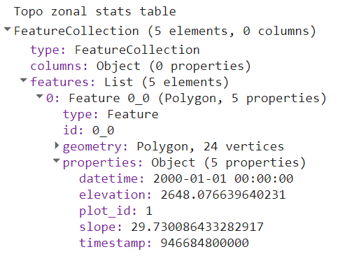
Fig. F5.2.2 Sample points and topographic slope. Elevation and slope values for regions intersecting each buffered point are reduced and attached as properties of the points. |
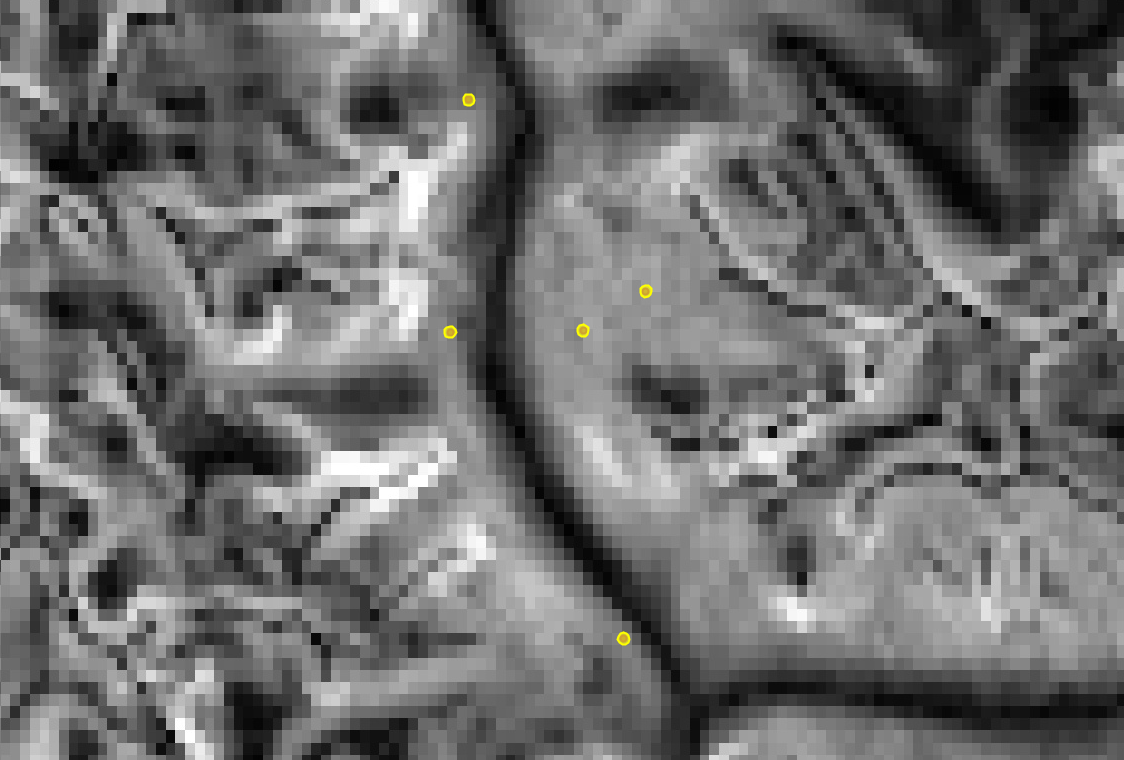
Table F5.2.3 Example output from zonalStats organized as a table. Rows correspond to collection features and columns are feature properties. Note that elevation and slope values in this table are rounded to the nearest tenth for brevity.
plot_id | timestamp | datetime | elevation | slope |
1 | 946684800000 | 2000-01-01 00:00:00 | 2648.1 | 29.7 |
2 | 946684800000 | 2000-01-01 00:00:00 | 2888.2 | 33.9 |
3 | 946684800000 | 2000-01-01 00:00:00 | 3267.8 | 35.8 |
4 | 946684800000 | 2000-01-01 00:00:00 | 2790.7 | 25.1 |
5 | 946684800000 | 2000-01-01 00:00:00 | 2559.4 | 29.4 |
Section 3.2. MODIS Time Series
A time series of MODIS eight-day surface reflectance composites demonstrates how to calculate zonal statistics for a multiband ImageCollection that requires no preprocessing, such as cloud masking or computation. Note that there is no built-in function for performing region reductions on ImageCollection objects. The zonalStats function that we are using for reduction is mapping the reduceRegions function over an ImageCollection.
Section 3.2.1. Buffer the Points
In this example, suppose the point collection represents center points for field plots that are 100 m x 100 m, and apply a 50 m radius buffer to the points to match the size of the plot. Since we want zonal statistics for square plots, set the second argument of the bufferPoints function to true, so that the bounds of the buffered points are returned.
var ptsModis=pts.map(bufferPoints(50, true)); |
Section 3.2.2. Calculate Zonal Statistic
Import the MODIS 500 m global eight-day surface reflectance composite collection and filter the collection to include data for July, August, and September from 2015 through 2019.
var modisCol=ee.ImageCollection('MODIS/006/MOD09A1') |
Reduce each image in the collection by each plot according to the following parameters. Note that this time the reducer is defined as the neighborhood median (ee.Reducer.median) instead of the default mean, and that scale, CRS, and properties for the datetime are explicitly defined.
// Define parameters for the zonalStats function. |
The result is a feature collection with a feature for all combinations of plots and images. Interpreted as a table, the result has 200 rows (5 plots times 40 images) and as many columns as there are feature properties. Feature properties include those from the plot asset and the image, and any associated non-system image properties. Note that the printed results are limited to the first 50 features for brevity.
Section 3.3. Landsat Time Series
This example combines Landsat surface reflectance imagery across three instruments: Thematic Mapper (TM) from Landsat 5, Enhanced Thematic Mapper Plus (ETM+) from Landsat 7, and Operational Land Imager (OLI) from Landsat 8.
The following section prepares these collections so that band names are consistent and cloud masks are applied. Reflectance among corresponding bands are roughly congruent for the three sensors when using the surface reflectance product; therefore the processing steps that follow do not address inter-sensor harmonization. Review the current literature on inter-sensor harmonization practices if you'd like to apply a correction.
Section 3.3.1. Prepare the Landsat Image Collection
First, define the function to mask cloud and shadow pixels (See Chap. F4.3 for more detail on cloud masking).
// Mask clouds from images and apply scaling factors. |
Next, define functions to select and rename the bands of interest for the Operational Land Imager (OLI) aboard Landsat 8, and for the TM/ETM+ imagers aboard earlier Landsats. This is important because the band numbers are different for OLI and TM/ETM+, and it will make future index calculations easier.
// Selects and renames bands of interest for Landsat OLI. |
Combine the cloud mask and band renaming functions into preparation functions for OLI and TM/ETM+. Add any other sensor-specific preprocessing steps that you’d like to the functions below.
// Prepares (cloud masks and renames) OLI images. |
Get the Landsat surface reflectance collections for OLI, ETM+, and TM sensors. Filter them by the bounds of the point feature collection and apply the relevant image preparation function.
var ptsLandsat=pts.map(bufferPoints(15, true)); |
Merge the prepared sensor collections.
var landsatCol=oliCol.merge(etmCol).merge(tmCol); |
Section 3.3.2. Calculate Zonal Statistics
Reduce each image in the collection by each plot according to the following parameters. Note that this example defines the imgProps and imgPropsRename parameters to copy over and rename just two selected image properties: Landsat image ID and the satellite that collected the data. It also uses the max reducer, which, as an unweighted reducer, will return the maximum value from pixels that have their centroid within the buffer (see Sect. 4.1 below for more details).
// Define parameters for the zonalStats function. |
The result is a feature collection with a feature for all combinations of plots and images.
Section 3.3.3. Dealing with Large Collections
If your browser times out, try exporting the results (as described in Chap. F6.2). It’s likely that point feature collections that cover a large area or contain many points (point-image observations) will need to be exported as a batch task by either exporting the final feature collection as an asset or as a CSV/shapefile/GeoJSON to Google Drive or GCS.
Here is how you would export the above Landsat image-point feature collection to an asset and to Google Drive. Run the following code, activate the Code Editor Tasks tab, and then click the Run button. If you don’t specify your own existing folder in Drive, the folder “EEFA_outputs” will be created.
Export.table.toAsset({ |
Code Checkpoint F52b. The book’s repository contains a script that shows what your code should look like at this point.
Section 4. Additional Notes
Section 4.1. Weighted Versus Unweighted Region Reduction
A region used for calculation of zonal statistics often bisects multiple pixels. Should partial pixels be included in zonal statistics? Earth Engine lets you decide by allowing you to define a reducer as either weighted or unweighted (or you can provide per-pixel weight specification as an image band). A weighted reducer will include partial pixels in the zonal statistic calculation by weighting each pixel's contribution according to the fraction of the area intersecting the region. An unweighted reducer, on the other hand, gives equal weight to all pixels whose cell center intersects the region; all other pixels are excluded from calculation of the statistic.
For aggregate reducers like ee.Reducer.mean and ee.Reducer.median, the default mode is weighted, while identifier reducers such as ee.Reducer.min and ee.Reducer.max are unweighted. You can adjust the behavior of weighted reducers by calling unweighted on them, as in ee.Reducer.mean.unweighted. You may also specify the weights by modifying the reducer with splitWeights; however, that is beyond the scope of this book.
Section 4.2. Copy Properties to Computed Images
Derived, computed images do not retain the properties of their source image, so be sure to copy properties to computed images if you want them included in the region reduction table. For instance, consider the simple computation of unscaling Landsat SR data:
// Define a Landsat image. |
Notice how the computed image does not have the source image's properties and only retains the bands information. To fix this, use the copyProperties function to add desired source properties to the derived image. It is best practice to copy only the properties you really need because some properties, such as those containing geometry objects, lists, or feature collections, can significantly increase the computational burden for large collections.
// Subset the reflectance bands and unscale them, keeping selected |
Now selected properties are included. Use this technique when returning computed, derived images in a mapped function, and in single-image operations.
Section 4.3. Understanding Which Pixels are Included in Polygon Statistics
If you want to visualize what pixels are included in a polygon for a region reducer, you can adapt the following code to use your own region (by replacing geometry), dataset, desired scale, and CRS parameters. The important part to note is that the image data you are adding to the map is reprojected using the same scale and CRS as that used in your region reduction (see Fig. F5.2.3).
// Define polygon geometry. |
The count reducer will return how many pixel centers are overlapped by the polygon region, which would be the number of pixels included in any unweighted reducer statistic. You can also visualize which pixels will be included in the reduction by using the toCollection reducer on a latitude/longitude image and adding resulting coordinates as feature geometry. Be sure to specify CRS and scale for both the region reducers and the reprojected layer added to the map (see bullet list below for more details).
// A count reducer will return how many pixel centers are overlapped by the |
Fig. F5.2.3 Identifying pixels used in zonal statistics. By mapping the image and vector together, you can see which pixels are included in the unweighted statistic. For this example, three pixels would be included in the statistic because the polygon covers the center point of three pixels. |

Code Checkpoint F52c. The book’s repository contains a script that shows what your code should look like at this point.
Finally, here are some notes on CRS and scale:
- Earth Engine runs reduceRegion using the projection of the image's first band if the CRS is unspecified in the function. For imagery spanning multiple UTM zones, for example, this would lead to different origins. For some functions Earth Engine uses the default EPSG:4326. Therefore, when the opportunity is presented, such as by the reduceRegion function, it is important to specify the scale and CRS explicitly.
- The Map default CRS is EPSG:3857. When looking closely at pixels on the map, the data layer scale and CRS should also be set explicitly. Note that zooming out after setting a relatively small scale when reprojecting may result in memory and/or timeout errors because optimized pyramid layers for each zoom level will not be used.
- Specifying the CRS and scale in both the reduceRegion and addLayer functions allows the map visualization to align with the information printed in the Console.
- The Earth Engine default, WGS 84 lat long (EPSG:4326), is a generic CRS that works worldwide. The code above reprojects to EPSG:5070, North American Equal Albers, which is a CRS that preserves area for North American locations. Use the CRS that is best for your use case when adapting this to your own project, or maintain (and specify) the CRS of the image using, for example, crs: 'img.projection().crs()'.
Synthesis
Question 1. Look at the MODIS example (Sect. 3.2), which uses the median reducer. Try modifying the reducer to be unweighted, either by specifying unweighted or using an identifier reducer like max. What happens, and why?
Question 2. Calculate zonal statistics for your own buffered points or polygons using a raster and reducer of interest. Be sure to consider the spatial scale of the raster and whether a weighted or unweighted reducer would be more appropriate for your interests.
If the point or polygon file is stored in a local shapefile or CSV file, first upload the data to your Earth Engine assets. All columns in your vector file, such as the plot name, will be retained through this process. Once you have an Earth Engine table asset ready, import the asset into your script by hovering over the name of the asset and clicking the arrow at the right side, or by calling it in your script with the following code.
var pts=ee.FeatureCollection('users/yourUsername/yourAsset'); |
If you prefer to define points or polygons dynamically rather than loading an asset, you can add them to your script using the geometry tools. See Chap. F2.1 and F5.0 for more detail on adding and creating vector data.
Question 3. Try the code from Sect. 4.3 using the MODIS data and the first point from the pts variable. Among other modifications, you will need to create a buffer for the point, take a single MODIS image from the collection, and change visualization parameters.
- Think about the CRS in the code: The code reprojects to EPSG:5070, but MODIS is collected in the sinusoidal projection SR-ORG:6974. Try that CRS and describe how the image changes.
- Is the count reducer weighted or unweighted? Give an example of a circumstance to use a weighted reducer and an example for an unweighted reducer. Specify the buffer size you would use and the spatial resolution of your dataset.
Question 4. In the examples above, only a single ee.Reducer is passed to the zonalStats function, which means that only a single statistic is calculated (for example, zonal mean or median or maximum). What if you want multiple statistics—can you alter the code in Sect. 3.1 to (1) make the point buffer 500 instead of 45; (2) add the reducer parameter to the params dictionary; and (3) as its argument, supply a combined ee.Reducer that will calculate minimum, maximum, standard deviation, and mean statistics?
To achieve this you’ll need to chain several ee.Reducer.combine functions together. Note that if you accept all the individual ee.Reducer and ee.Reducer.combine function defaults, you’ll run into two problems related to reducer weighting differences, and whether or not the image inputs are shared among the combined set of reducers. How can you manipulate the individual ee.Reducer and ee.Reducer.combine functions to achieve the goal of calculating multiple zonal statistics in one call to the zonalStats function?
Conclusion
In this chapter, you used functions containing optional parameters to extract raster values for collocated points. You also learned how to buffer points, and apply weighted and unweighted reducers to get different types of zonal statistics. These functions were applied to three examples that differed by raster dataset, reducer, spatial resolution, and scale. Lastly, you covered related topics like weighting of reducers and buffer visualization. Now you’re ready to apply these ideas to your own work!
Feedback
To review this chapter and make suggestions or note any problems, please go now to bit.ly/EEFA-review. You can find summary statistics from past reviews at bit.ly/EEFA-reviews-stats.
References
Cloud-Based Remote Sensing with Google Earth Engine. (n.d.). CLOUD-BASED REMOTE SENSING WITH GOOGLE EARTH ENGINE. https://www.eefabook.org/
Cloud-Based Remote Sensing with Google Earth Engine. (2024). In Springer eBooks. https://doi.org/10.1007/978-3-031-26588-4
Cansler CA, McKenzie D (2012) How robust are burn severity indices when applied in a new region? Evaluation of alternate field-based and remote-sensing methods. Remote Sens 4:456–483. https://doi.org/10.3390/rs4020456
Miller JD, Thode AE (2007) Quantifying burn severity in a heterogeneous landscape with a relative version of the delta Normalized Burn Ratio (dNBR). Remote Sens Environ 109:66–80. https://doi.org/10.1016/j.rse.2006.12.006