Terrestrial Applications part 2

Conservation I Assessing the spatial relationship between burned area and precipitation

Cloud-Based Remote Sensing with Google Earth Engine

Fundamentals and Applications

Part A3: Terrestrial Applications

Earth’s terrestrial surface is analyzed regularly by satellites, in search of both change and stability. These are of great interest to a wide cross-section of Earth Engine users, and projects across large areas illustrate both the challenges and opportunities for life on Earth. Chapters in this Part illustrate the use of Earth Engine for disturbance, understanding long-term changes of rangelands, and creating optimum study sites.

Chapter A3.9: Conservation Applications - Assessing the spatial relationship between burned area and precipitation

Authors

Harriet Branson and Chelsea Smith

Overview

The purpose of this chapter is to introduce the need for fire and rainfall trend monitoring to inform conservation management practices.

Practical conservation requires an understanding of key environmental factors such as fire and rainfall, which impact the amount of forage and habitat available for a variety of species. This chapter will guide you through how to create fire and rainfall time series and visualize this data. At the end of this chapter, you will be able to present this information in an accessible way on a graph to help inform conservation management practices such as early burning and supplementary feeding.

Learning Outcomes

Understanding why fire and rainfall trends are useful in conservation management.
Creating a time series of burned areas.
Writing a function to map areal mean rainfall calculations over an ImageCollection.
Generating an interactive graph displaying fire and rainfall trends over a 10-year period.

Helps if you know how to:

Import images and image collections, filter, and visualize (Part F1).
Create a graph using ui.Chart (Chap. F1.3).
Summarize an image with reduceRegion (Chap. F3.1).
Write a function and map it over an ImageCollection (Chap. F4.0).
Work with CHIRPS rainfall data (Chap. F4.2).
Mask cloud, cloud shadow, snow/ice, and other undesired pixels (Chap. F4.3).

Github Code link for all tutorials

This code base is collection of codes that are freely available from different authors for google earth engine.

Github Source

Introduction to Theory

Globally, biodiversity is under threat from changing climates, habitat loss, and fragmentation. Conservation work to protect, manage and restore ecosystems is vitally important to maintain global biodiversity, which supports climate regulation and a host of other ecosystem services we depend upon (Reddy 2021).

Remote sensing offers a valuable tool to collect, analyze, and display data over an entire ecosystem. Environmental variables such as fire and rainfall have direct impacts on habitat and forage availability. Monitoring of these variables can help inform conservation, such as fire management to reduce the severity of fires and amount of habitat lost (Ribeiro et al. 2021). Monitoring rainfall patterns can help conservationists understand which climate conditions species prefer in their habitats and if the conditions are at risk of changing (Pinto-Ledezma and Cavender-Bares 2021).

In this chapter we will see how using the Earth Engine platform allows conservationists to scope the fire and rainfall conditions for any site using global datasets. The data we visualize is being directly used in real-world conservation by informing fire management, as well as indirectly through the identification of climate conditions to which species are adapted.

Practicum

Section 1. Assess Area of Interest

The first step is to upload and explore the area of interest. Northern Mozambique’s Niassa Reserve is home to 40% of the country’s entire elephant population, and is a haven for two of Africa’s threatened carnivores, lion and wild dog. Fire is a key ecological process in forested savanna ecosystems that are prevalent in the Niassa Reserve, and the knowledge of the fire regime is an important factor in forest fire management. Our area of interest (AOI) has very stark wet and dry seasons; take a look at the satellite imagery basemap that shows the landscape in the wet season.

// ** Upload the area of interest ** //
var AOI=ee.Geometry.Polygon([
[
[37.72, -11.22],
[38.49, -11.22],
[38.49, -12.29],
[37.72, -12.29]
]
]);
Map.centerObject(AOI, 9);
Map.addLayer(AOI,{
color: 'white'
}, 'Area of interest');

Section 2. Load the MODIS Burned Area Dataset

Next, we will use the MCD64A1 dataset, which is a global layer representing burned area at 500 m resolution from 2001 to the present. The layer is also accompanied by a band named 'BurnDate', which enables you to disaggregate into daily fire data.

First, we will filter the MODIS ImageCollection based on the timespan requirements. We are looking at fire patterns over the past 10 years. The MCD64A1 dataset comes with three main bands, 'BurnDate', 'Uncertainty', and 'QA' (quality assurance). In this case, we select only the 'BurnDate' band, which associates each pixel of burned area with a day-of-year value.

// ** MODIS Monthly Burn Area ** //

// Load in the MODIS Monthly Burned Area dataset.
var dataset=ee.ImageCollection('MODIS/006/MCD64A1')
// Filter based on the timespan requirements.
.filter(ee.Filter.date('2010-01-01', '2021-12-31'));

// Select the BurnDate band from the images in the collection.
var MODIS_BurnDate=dataset.select('BurnDate');

Next we can create the function that will calculate the area of pixels associated with each day. The function is structured so that it will map over each image in the MODIS_BurnDate ImageCollection. It begins by using the command pixelArea, which calculates the area of each pixel in square meters. To limit the calculation to specifically burned areas, we need to use updateMask with our input img as the variable. Because we want our final area calculation to be in square kilometers instead of square meters, we divide the value by 1,000,000 (1e6).

The reduceRegion command gathers the sum of burned area within our input area of interest at the correct scale of the input image (500 m for our MODIS_BurnDate collection). After this, the getNumber command recalls the area calculation per image per day of year and appends it as a new band area on the ImageCollection.

Since the MODIS ImageCollection has a 'system:time_start' embedded within each image, we can select the area band and continue without the 'BurnDate'.

// A function that will calculate the area of pixels in each image by date.
var addArea=function(img) {
var area=ee.Image.pixelArea()
.updateMask(
img
) // Limit area calculation to areas that have burned data.
.divide(1e6) // Divide by 1,000,000 for square kilometers.
.clip(AOI) // Clip to the input geometry.
.reduceRegion({
reducer: ee.Reducer.sum(),
geometry: AOI,
scale: 500,
bestEffort: true
}).getNumber(
'area'
); // Retrieve area from the reduce region calculation.
// Add a new band to each image in the collection named area.
return img.addBands(ee.Image(area).rename('area'));
};

// Apply function on image collection.
var burnDateArea=MODIS_BurnDate.map(addArea);

// Select only the area band as we are using system time for date.
var burnedArea=burnDateArea.select('area');

To show the total amount of burned area over the past 10 years, we can plot this on a time-series graph. By defining the xProperty with 'system:time_start' for the date variable on this graph, we can plot the total area burned with time.

// Create a chart that shows the total burned area over time.
var burnedAreaChart=
ui.Chart.image
.series({
imageCollection: burnedArea, // Our image collection.
region: AOI,
reducer: ee.Reducer.mean(),
scale: 500,
xProperty: 'system:time_start' // time
})
.setSeriesNames(['Area']) // Label for legend.
.setOptions({
title: 'Total monthly area burned in AOI',
hAxis:{
title: 'Date', // The x axis label.
format: 'YYYY', // Years only for date format.
gridlines: {
count: 12
},
titleTextStyle:{
italic: false,
bold: true
}
},
vAxis:{
title: 'Total burned area (km²)', // The y-axis label
maxValue: 2250, // The bounds for y-axis
minValue: 0,
titleTextStyle:{
italic: false,
bold: true
}
},
lineWidth: 1.5,
colors: ['d74b46'], // The line color
});
print(burnedAreaChart);

Code Checkpoint A39a. The book’s repository contains a script that shows what your code should look like at this point.

Question 1. We have calculated the area burned in square kilometers; which line of code would you have to change, and how, to calculate the area burned in hectares?

Question 2. By hovering your mouse over the graph, which month has the greatest area burnt, and does this vary year on year?

Question 3. The most appropriate fire dataset and analysis to use for your study will vary depending on location and scale of analysis. If you wanted to understand the impact of fires on koala habitat in southern Australia, what would be the most appropriate analysis? Hint: Consider the analysis run in Chap. A3.1 and the work by Bonney et al. (2020).

Section 3. Areal Mean Rainfall Time Series

To inform habitat management and further understand fire patterns within northern Mozambique, we have to also consider patterns in rainfall. To do this, we will use the Climate Hazards Group InfraRed Precipitation with Station (CHIRPS) Precipitation dataset. This dataset measures precipitation levels every five days from 1981 to present day at 500 m resolution to make a long-term quasi-global dataset.

First, we will define our temporal range (matching our burned area data) from 2010 to 2021, and set the advancing dates from these years. After this, we create a sequence of years and months that will be used to filter the dataset chronologically.

After setting these parameters, filter the CHIRPS dataset using the start and end date, and sort chronologically in descending order using the same 'system:time_start' property used in Sect. 1. Filter the bounds to the AOI, and select the precipitation band from the ImageCollection.

// Load in the CHIRPS rainfall pentad dataset.
var chirps=ee.ImageCollection('UCSB-CHG/CHIRPS/PENTAD');

// Define the temporal range
var startyear=2010;
var endyear=2021;

// Set the advancing dates from the temporal range.
var startdate=ee.Date.fromYMD(startyear, 1, 1);
var enddate=ee.Date.fromYMD(endyear, 12, 31);

// Create a list of years
var years=ee.List.sequence(startyear, endyear);
// Create a list of months
var months=ee.List.sequence(1, 12);

// Filter the dataset based on the temporal range.
var Pchirps=chirps.filterDate(startdate, enddate)
.sort('system:time_start',
false) // Sort chronologically in descending order.
.filterBounds(AOI) // Filter to AOI
.select('precipitation'); // Select precipitation band

Once the dataset has been filtered, we can calculate the monthly precipitation using a function. The function maps the input, y, over the list of years generated above. The function then returns the total precipitation for the month, alongside a date variable and the 'system:time_start' property. The command millis is used to keep the system number that refers to the date collected.

Print the ImageCollection for checking.

// Calculate the precipitation per month.
var MonthlyRainfall=ee.ImageCollection.fromImages(
years.map(function(
y
){ // Using the list of years based on temporal range.
return months.map(function(m){
var w=Pchirps.filter(ee.Filter
.calendarRange(y, y, 'year'))
.filter(ee.Filter.calendarRange(m, m,
'month'))
.sum(); // Calculating the sum for the month
return w.set('year', y)
.set('month', m)
.set('system:time_start', ee.Date
.fromYMD(y, m, 1).millis()
) // Use millis to keep the system time number.
.set('date', ee.Date.fromYMD(y, m,
1));
});
}).flatten());
// Print the image collection.
print('Monthly Precipitation Image Collection', MonthlyRainfall);

Once the monthly precipitation levels have been calculated, we can use a reducer to calculate the mean total rainfall across our AOI, also known as the areal mean rainfall (AMR), and plot these on a time series graph. This process is very similar to the burned area chart in Sect. 2.

// ** Chart: CHIRPS Precipitation ** //

// Create a chart displaying monthly rainfall over a temporal range.
var monthlyRainfallChart=
ui.Chart.image
.series({
imageCollection: MonthlyRainfall.select(
'precipitation'), // Select precipitation band
region: AOI,
reducer: ee.Reducer
.mean(), // Use mean reducer to calculate AMR
scale: 500,
xProperty: 'system:time_start' // Use system time start for x-axis
})
.setSeriesNames(['Precipitation']) // /The label legend
.setOptions({
title: 'Total monthly precipitation in AOI', // Add title
hAxis: {
title: 'Date',
format: 'YYYY', // Year only date format
gridlines:{
count: 12
},
titleTextStyle:{
italic: false,
bold: true
}
},
vAxis:{
title: 'Precipitation (mm)', // The y-axis label
maxValue: 450, // The bounds for y-axis
minValue: 0,
titleTextStyle:{
italic: false,
bold: true
}
},
lineWidth: 1.5,
colors: ['4f5ebd'],
});
print(monthlyRainfallChart);

Print the monthly rainfall chart. Using the chart, we can see which months receive rainfall, and can categorize these as the wet season. With data from the chart, we will categorize any month that receives over 5 mm of rainfall as a wet season month. We can then calculate total seasonal rainfall across our AOI by aggregating wet season months together.

// 2010/2011 wet season total
var year=2010; // Adjust year
var startDate=ee.Date.fromYMD(year, 11, 1); // Adjust months/days
var endDate=ee.Date.fromYMD(year + 1, 5, 31); // Adjust months/days
var filtered=chirps
.filter(ee.Filter.date(startDate, endDate));
var Rains10_11Total=filtered.reduce(ee.Reducer.sum()).clip(AOI);

// 2011/2012 wet season total
var year=2011; // Adjust year
var startDate=ee.Date.fromYMD(year, 11, 1); // Adjust months/days
var endDate=ee.Date.fromYMD(year + 1, 5, 31); // Adjust months/days
var filtered=chirps
.filter(ee.Filter.date(startDate, endDate));
var Rains11_12Total=filtered.reduce(ee.Reducer.sum()).clip(AOI);

Question 4. Classify the remaining wet seasons using the areal mean rainfall chart, and calculate the total seasonal rainfall over the AOI using the code you have just learned, to calculate wet seasons in 2010–2011 and 2011–2012.

Question 5. We have created a 10-year time series. Is this a long enough time period to start to consider changes in rainfall patterns?

Code Checkpoint A39b. The book’s repository contains a script that shows what your code should look like at this point.

Section 4. Visualizing Fire and Rainfall Time Series

Now that we have visualized patterns in both burned area and precipitation separately, it is important to assess these patterns together. To do this, we need to combine the two image collections in order to plot them on the same graph.

Once they are combined, we can begin creating a multi-variable time-series chart. By keeping the 'system:time_start' property on both sets of image collections, we are able to easily plot each variable temporally. Following this, we set both series’ names and set interpolateNulls to true to provide continuous precipitation data that can be plotted alongside the near daily burned area data.

To enable two y-axes, we need to set some series parameters. By defining our targetAxisIndex as 0 and 1, we can then set our vAxes to match, using two sets of parameters with different labels and different bounds for ease of plotting. This is useful since the burned area and precipitation datasets have different minimum and maximum values, so it would be difficult to analyze on the same axis.

You can print the chart to the Console for export if necessary, but for interactivity we will add it to the map later.

// ** Combine: CHIRPS Average Rainfall & MODIS Monthly Burn ** //

// Combine the two image collections for joint analysis
var bpMerged=burnedArea.merge(MonthlyRainfall);
print('Merged image collection', bpMerged);

// ** Chart: CHIRPS Average Rainfall & MODIS Monthly Burn ** //
// Plot the two time series on a graph
var bpChart=
ui.Chart.image.series({
imageCollection: bpMerged, // The merged image collection
region: AOI,
reducer: ee.Reducer.mean(),
scale: 500,
xProperty: 'system:time_start' // Use system time start for synchronous plotting
})
.setSeriesNames(['Burned Area', 'Precipitation']) // Label series
.setChartType('LineChart') // Define chart type
.setOptions({
title: 'Relationship between burned area and rainfall in Chuilexi',
interpolateNulls: true, // Interpolate nulls to provide continuous data
series:{ // Use two sets of series with a target axis to create the two y-axes needed for plotting
0:{ // 0 and 1 reference the vAxes settings below
targetAxisIndex: 0,
type: 'line',
lineWidth: 1.5,
color: 'd74b46'
},
1:{
targetAxisIndex: 1,
type: 'line',
lineWidth: 1.5,
color: '4f5ebd'
},
},
hAxis:{
title: 'Date',
format: 'YYYY',
gridlines:{
count: 12
},
titleTextStyle:{
italic: false,
bold: true
}
},
vAxes:{
0:{
title: 'Burned area (km²)', // Label left-hand y-axis
baseline: 0,
viewWindow:{
min: 0
},
titleTextStyle:{
italic: false,
bold: true
}
},
1:{
title: 'Precipitation (mm)', // Label right-hand y-axis
baseline: 0,
viewWindow:{
min: 0
},
titleTextStyle:{
italic: false,
bold: true
}
},
},
curveType: 'function' // For smoothing
});
bpChart.style().set({
position: 'bottom-right',
width: '492px',
height: '300px'
});

Once we have created our final chart that displays burned area and precipitation, we can build some legends on the map for the spatial data. Using two different functions, we can create a horizontal legend with a set gradient palette and custom markers that correspond to the precipitation data.

The burned area legend is simpler in that we are creating a square of red to indicate that any pixel marked red on the image was burned at that particular time point.

// ** Legend: Rainfall ** //
var rain_palette=['#ffffcc', '#a1dab4', '#41b6c4', '#2c7fb8',
'#253494'
];

function ColorBar(rain_palette){
return ui.Thumbnail({
image: ee.Image.pixelLonLat().select(0),
params:{
bbox: [0, 0, 1, 0.1],
dimensions: '300x15',
format: 'png',
min: 0,
max: 1,
palette: rain_palette,
},
style:{
stretch: 'horizontal',
margin: '0px 22px'
},
});
}

function makeRainLegend(lowLine, midLine, highLine, lowText, midText,
highText, palette){
var labelheader=ui.Label(
'Total precipitation in wet season (mm)',{
margin: '5px 17px',
textAlign: 'center',
stretch: 'horizontal',
fontWeight: 'bold'
});
var labelLines=ui.Panel(
[
ui.Label(lowLine,{
margin: '-4px 21px'
}),
ui.Label(midLine,{
margin: '-4px 0px',
textAlign: 'center',
stretch: 'horizontal'
}),
ui.Label(highLine,{
margin: '-4px 21px'
})
],
ui.Panel.Layout.flow('horizontal'));
var labelPanel=ui.Panel(
[
ui.Label(lowText,{
margin: '0px 14.5px'
}),
ui.Label(midText,{
margin: '0px 0px',
textAlign: 'center',
stretch: 'horizontal'
}),
ui.Label(highText,{
margin: '0px 1px'
})
],
ui.Panel.Layout.flow('horizontal'));
return ui.Panel({
widgets: [labelheader, ColorBar(rain_palette),
labelLines, labelPanel
],
style:{
position: 'bottom-left'
}
});
}
Map.add(makeRainLegend('|', '|', '|', '0', '250', '500', ['#ffffcc',
'#a1dab4', '#41b6c4', '#2c7fb8', '#253494'
]));

// ** Legend: Burned area ** //
var burnLegend=ui.Panel({
style:{
position: 'top-left',
padding: '8px 15px'
}
});

var makeRow=function(color, name){
var colorBox=ui.Label({
style:{
backgroundColor: '#' + color,
padding: '10px',
margin: '0 10px 0 0'
}
});
var description=ui.Label({
value: name,
style: {
margin: 'o o 6px 6px'
}
});
return ui.Panel({
widgets: [colorBox, description],
layout: ui.Panel.Layout.Flow('horizontal')
});
};

var burnPalette=['FF0000'];
var names=['Burned area'];
for (var i=0; i < 1; i++){
burnLegend.add(makeRow(burnPalette[i], names[i]));
}
Map.add(burnLegend);

Now that we have our legends complete, we can add our double variable time-series chart to the map, and center the map on our area of interest.

Map.centerObject(AOI, 9); // Centre the map on the AOI
Map.add(
bpChart
); // Add the merged burned area & precipitation chart to the map

While visualizing the data on a static chart is useful for further analysis and identifying patterns, it is also useful to see the spatial data corresponding to a particular date or fire. To do this, we can add an interactive element to the chart. If you click a particular point on the chart, it will reveal the corresponding image for burned area and precipitation on the map.

To do this, we need to create a function that uses the burned area and precipitation chart (bpChart) and executes onClick, displaying the relevant data based on the input values. By utilizing the 'system:time_start' property, we can query the date, which will then be used to identify the first image (first) that appears within the list of images, within the area of interest. We can then format the legend box within the map so that it shows the date and time of the layer selected.

Following this, we can set the symbology of each layer (burned area in red, and the precipitation color gradient indicated in the legend settings), and display the relevant layer with the date text string on the map.

// ** Chart: Adding an interactive query ** //

// Add a function where if you click on a point in the map it displays the burned area and rainfall for that date
bpChart.onClick(function(xValue, yValue, seriesName){
if (!xValue) return;
// Show layer for date selected on the chart
var equalDate=ee.Filter.equals('system:time_start',
xValue);
// Search for the layer in the image collection that links to the selected date
var classificationB=ee.Image(MODIS_BurnDate.filter(
equalDate).first()).clip(AOI).select('BurnDate');
var classificationR=ee.Image(MonthlyRainfall.filter(
equalDate).first()).clip(AOI).select(
'precipitation');
var burnImage=ee.Image(MODIS_BurnDate.filter(equalDate)
.first());
var date_string=new Date(xValue).toLocaleString(
'en-EN',{
dateStyle: 'full'
});
var rainImage=ee.Image(MonthlyRainfall.filter(equalDate)
.first());
var date_stringR=new Date(xValue).toLocaleString(
'en-EN',{
dateStyle: 'full'
});
// Reset the map layers each time a new date is clicked
Map.layers().reset([classificationB]);
Map.layers().reset([classificationR]);
var visParamsBurnLayer={ // Visualisation for burned area
min: 0,
max: 365,
palette: ['red']
};
var visParamsRainLayer={ // Visualisation for rain
min: 0,
max: 450,
palette: ['#ffffcc', '#a1dab4', '#41b6c4',
'#2c7fb8', '#253494'
]
};
// Add the layers to the map
Map.addLayer(classificationR, visParamsRainLayer,
'Total monthly rainfall on [' + date_string + ']');
Map.addLayer(classificationB, visParamsBurnLayer,
'Burned area on [' + date_string + ']');
});

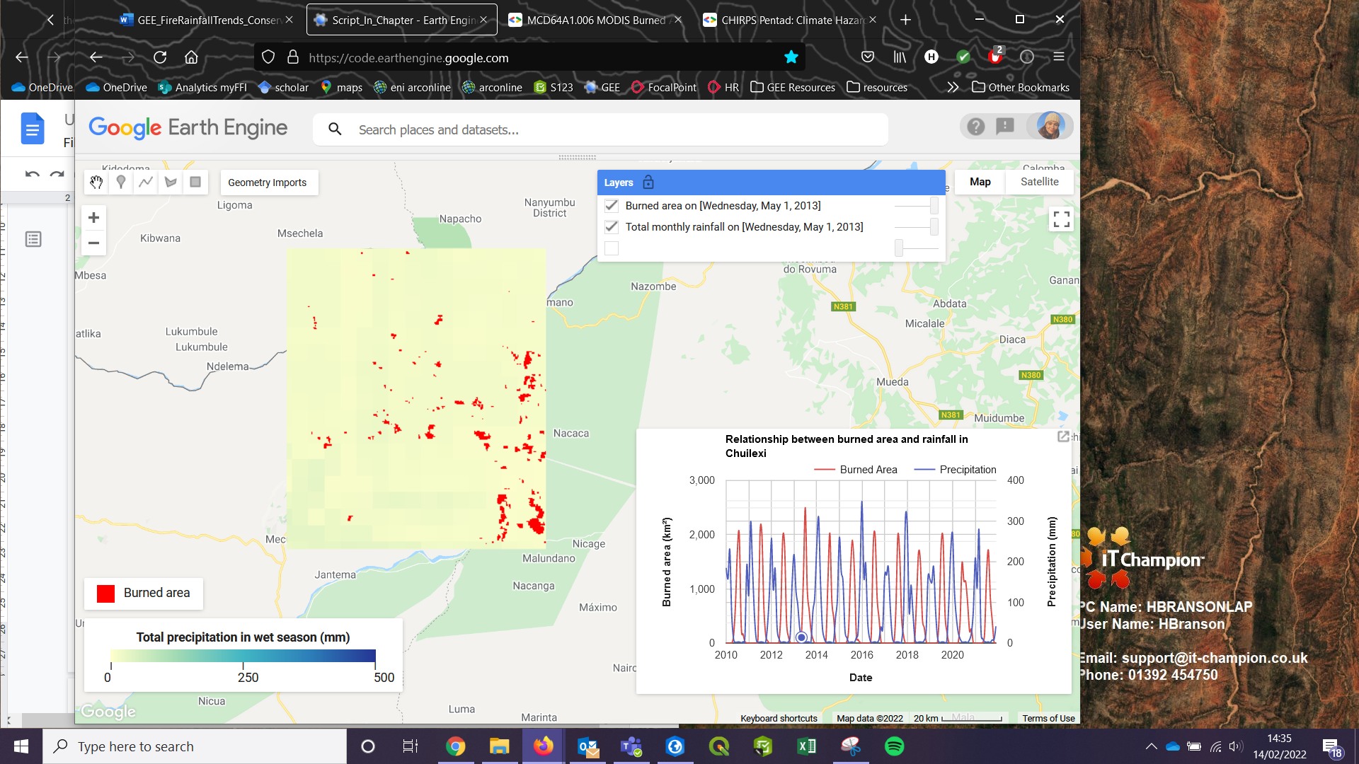
Fig. A3.9.1 The final result of the code once you have clicked on the chart to select a month to display, here showing the burned area and total precipitation at the beginning of the dry season in May 2021

Code Checkpoint A39c. The book’s repository contains a script that shows what your code should look like at this point.

Question 6. Considering the importance of environmental variables in conservation work, what other datasets and common earth observation analysis could provide data to inform conservation management?

Synthesis

In this chapter, you have learned how to create a time series of burned area, using the global MODIS burned area product. You also calculated areal mean rainfall using the CHIRPS dataset, and graphed total seasonal rainfall using your time-series chart. Additionally, you can now merge two image collections to show two variables on one interactive chart in the Earth Engine map.

With the code you have learned in this chapter, you can now create area burned and areal mean rainfall time series for your own region of interest anywhere in the world. Recreate the analysis in a different environment, and consider extending the time series over a longer period; can you detect any trends?

Monitoring vegetation is also important in conservation and can be significantly impacted by fire and rainfall trends. Try to modify the code you have learned to calculate areal mean NDVI from the NOAA CDR AVHRR daily NDVI dataset. Can you add this as another variable in the interactive chart?

Conclusion

In this chapter we understand and map the dynamic relationship between fire and rainfall, and how this can influence conservation action and land management needs. We began by mapping burned areas using MODIS Burned Area Monthly Global 500 m to understand how much of, and where, the landscape is affected by burning. Following this, we understood how to access rainfall data and calculate areal mean rainfall, plotting this on a graph to understand changes and patterns over time. By combining the burned area and rainfall data, we can see how rainfall (or lack thereof) can exacerbate burning, and begin to spot patterns in the landscape. This analysis, which would often be undertaken in the field or by hand using satellite imagery, is made accessible via Earth Engine—not only because we can perform this on a workstation that only requires an internet connection rather than computing power, but also because Earth Engine generates quick, consistent results that can inform conservation management practices.

Feedback

To review this chapter and make suggestions or note any problems, please go now to bit.ly/EEFA-review. You can find summary statistics from past reviews at bit.ly/EEFA-reviews-stats.

References

Cloud-Based Remote Sensing with Google Earth Engine. (n.d.). CLOUD-BASED REMOTE SENSING WITH GOOGLE EARTH ENGINE. https://www.eefabook.org/

Cloud-Based Remote Sensing with Google Earth Engine. (2024). In Springer eBooks. https://doi.org/10.1007/978-3-031-26588-4

Bonney MT, He Y, Myint SW (2020) Contextualizing the 2019–20 Kangaroo Island bushfires: Quantifying landscape-level influences on past severity and recovery with Landsat and Google Earth Engine. Remote Sens 12:1–32. https://doi.org/10.3390/rs12233942

Holden ZA, Swanson A, Luce CH, et al (2018) Decreasing fire season precipitation increased recent Western US forest wildfire activity. Proc Natl Acad Sci USA 115:E8349–E8357. https://doi.org/10.1073/pnas.1802316115

Nhongo E, Fontana D, Guasselli L (2020) Spatio-temporal patterns of wildfires in the Niassa Reserve –Mozambique, using remote sensing data. bioRxiv 1–7. https://doi.org/10.1101/2020.01.16.908780

Pinto-Ledezma JN, Cavender-Bares J (2021) Predicting species distributions and community composition using satellite remote sensing predictors. Sci Rep 11:1–12. https://doi.org/10.1038/s41598-021-96047-7

Reddy CS (2021) Remote sensing of biodiversity: What to measure and monitor from space to species? Biodivers Conserv 30:2617–2631. https://doi.org/10.1007/s10531-021-02216-5

Ribeiro NS, Armstrong AH, Fischer R, et al (2021) Prediction of forest parameters and carbon accounting under different fire regimes in Miombo woodlands, Niassa Special Reserve, Northern Mozambique. For Policy Econ 133:102625. https://doi.org/10.1016/j.forpol.2021.102625