Cloud-Based Remote Sensing with Google Earth Engine

Fundamentals and Applications

Part F4: Interpreting Image Series

One of the paradigm-changing features of Earth Engine is the ability to access decades of imagery without the previous limitation of needing to download all the data to a local disk for processing. Because remote-sensing data files can be enormous, this used to limit many projects to viewing two or three images from different periods. With Earth Engine, users can access tens or hundreds of thousands of images to understand the status of places across decades.

Chapter F4.7: Interpreting Time Series with CCDC

Authors 

Paulo Arévalo, Pontus Olofsson

Overview

Continuous Change Detection and Classification (CCDC) is a land change monitoring algorithm designed to operate on time series of satellite data, particularly Landsat data. This chapter focuses on the portion that is the change detection component (CCD); you will learn how to run the algorithm, interpret its outputs, and visualize coefficients and change information.

Learning Outcomes

• Exploring pixel-level time series of Landsat observations, as well as the temporal segments that CCDC fits to the observations.
• Visualizing the coefficients of the temporal segments in space.
• Visualizing predicted images made from detected temporal segments.
• Visualizing change information.
• Using array image functions.
• Attaching user-defined metadata to an image when exporting.

Assumes you know how to:

• Import images and image collections, filter, and visualize (Part F1).
• Perform basic image analysis: select bands, compute indices, create masks (Part F2).
• Visualize images with a variety of false-color band combinations (Chap. F1.1).
• Interpret bands and indices in terms of land surface characteristics (Chap. F2.0).
• Work with array images (Chap. F3.1, Chap. F4.6).
• Interpret fitted harmonic models (Chap. F4.6).

Introduction to Theory 

“A time series is a sequence of observations taken sequentially in time. … An intrinsic feature of a time series is that, typically, adjacent observations are dependent. Time-series analysis is concerned with techniques for the analysis of this dependency.” This is the formal definition of time-series analysis by Box et al. (1994). In a remote sensing context, the observations of interest are measurements of radiation reflected from the surface of the Earth from the Sun or an instrument emitting energy toward Earth. Consecutive measurements made over a given area result in a time series of surface reflectance. By analyzing such time series, we can achieve a comprehensive characterization of ecosystem and land surface processes (Kennedy et al. 2014). The result is a shift away from traditional, retrospective change-detection approaches based on data acquired over the same area at two or a few points in time to continuous monitoring of the landscape (Woodcock et al. 2020). Previous obstacles related to data storage, preprocessing, and computing power have been largely overcome with the emergence of powerful cloud-computing platforms that provide direct access to the data (Gorelick et al. 2017). In this chapter, we will illustrate how to study landscape dynamics in the Amazon river basin by analyzing dense time series of Landsat data using the CCDC algorithm. Unlike LandTrendr (Chap. F4.5), which uses anniversary images to fit straight line segments that describe the spectral trajectory over time, CCDC uses all available clear observations. This has multiple advantages, including the ability to detect changes within a year and capture seasonal patterns, although at the expense of much higher computational demands and more complexity to manipulate the outputs, compared to LandTrendr.

Github Code link for all tutorials

This code base is collection of codes that are freely available from different authors for google earth engine.

Github Source

Practicum

Section 1. Understanding Temporal Segmentation with CCDC

Spectral change is detected at the pixel level by testing for structural breaks in a time series of reflectance. In Earth Engine, this process is referred to as “temporal segmentation,” as pixel-level time series are segmented according to periods of unique reflectance. It does so by fitting harmonic regression models to all spectral bands in the time series. The model-fitting starts at the beginning of the time series and moves forward in time in an “online” approach to change detection. The coefficients are used to predict future observations, and if the residuals of future observations exceed a statistical threshold for numerous consecutive observations, then the algorithm flags that a change has occurred. After the change, a new regression model is fit and the process continues until the end of the time series. The details of the original algorithm are described in Zhu and Woodcock (2014). We have created an interface-based tool (Arévalo et al. 2020) that facilitates the exploration of time series of Landsat observations and the CCDC results.

Code Checkpoint F47a. The book’s repository contains information about accessing the CCDC interface.

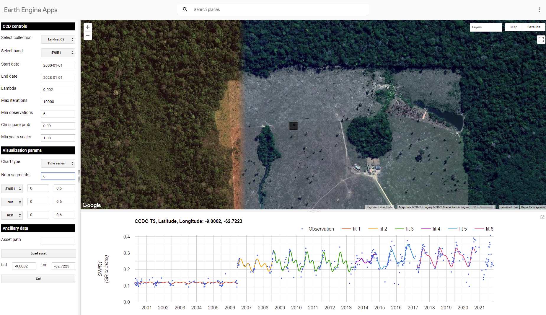
Once you have loaded the CCDC interface (Fig. F4.7.1), you will be able to navigate to any location, pick a Landsat spectral band or index to plot, and click on the map to see the fit by CCDC at the location you clicked. For this exercise, we will study landscape dynamics in the state of Rondônia, Brazil. We can use the panel on the left-bottom corner to enter the following coordinates (latitude, longitude): -9.0002, -62.7223. A point will be added in that location and the map will zoom in to it. Once there, click on the point and wait for the chart at the bottom to load. This example shows the Landsat time series for the first shortwave infrared (SWIR1) band (as blue dots) and the time segments (as colored lines) run using CCDC default parameters. The first segment represents stable forest, which was abruptly cut in mid-2006. The algorithm detects this change event and fits a new segment afterwards, representing a new temporal pattern of agriculture. Other subsequent patterns are detected as new segments are fitted that may correspond to cycles of harvest and regrowth, or a different crop. To investigate the dynamics over time, you can click on the points in the chart, and the Landsat images they correspond to will be added to the map according to the visualization parameters selected for the RGB combination in the left panel. Currently, changes made in that panel are not immediate but must be set before clicking on the map. 

Pay special attention to the characteristics of each segment. For example, look at the average surface reflectance value for each segment. The presence of a pronounced slope may be indicative of phenomena like vegetation regrowth or degradation. The number of harmonics used in each segment may represent seasonality in vegetation (either natural or due to agricultural practices) or landscape dynamics (e.g., seasonal flooding).

Question 1. While still using the SWIR1 band, click on a pixel that is forested. What do the time series and time segments look like?

Section 2. Running CCDC

The tool shown above is useful for understanding the temporal dynamics for a specific point. However, we can do a similar analysis for larger areas by first running the CCDC algorithm over a group of pixels. The CCDC function in Earth Engine can take any ImageCollection, ideally one with little or no noise, such as a Landsat ImageCollection where clouds and cloud shadows have been masked. CCDC contains an internal cloud masking algorithm and is rather robust against missed clouds, but the cleaner the data the better. To simplify the process, we have developed a function library that contains functions for generating input data and processing CCDC results. Paste this line of code in a new script:

For the current exercise, we will obtain an ImageCollection of Landsat 4, 5, 7, and 8 data (Collection 2 Tier 1) that has been filtered for clouds, cloud shadows, haze, and radiometrically saturated pixels. If we were to do this manually, we would retrieve each ImageCollection for each satellite, apply the corresponding filters and then merge them all into a single ImageCollection. Instead, to simplify that process, we will use the function getLandsat, included in the “Inputs” module of our utilities, and then filter the resulting ImageCollection to a small study region for the period between 2000 and 2020. The getLandsat function will retrieve all surface reflectance bands (renamed and scaled to actual surface reflectance units) as well as other vegetation indices. To simplify the exercise, we will select only the surface reflectance bands we are going to use, adding the following code to your script:

With the ImageCollection ready, we can specify the CCDC parameters and run the algorithm. For this exercise we will use the default parameters, which tend to work reasonably well in most circumstances. The only parameters we will modify are the breakpoint bands, date format, and lambda. We will set all the parameter values in a dictionary that we will pass to the CCDC function. For the break detection process we use all bands except for the blue and surface temperature bands ('BLUE' and 'TEMP', respectively). The minObservations default value of 6 represents the number of consecutive observations required to flag a change. The chiSquareProbability and minNumOfYearsScaler default parameters of 0.99 and 1.33, respectively, control the sensitivity of the algorithm to detect change and the iterative curve fitting process required to detect change. We set the date format to 1, which corresponds to fractional years and tends to be easier to interpret. For instance, a change detected in the middle day of the year 2010 would be stored in a pixel as 2010.5. Finally, we use the default value of lambda of 20, but we scale it to match the scale of the inputs (surface reflectance units), and we specify a maxIterations value of 10000, instead of the default of 25000, which might take longer to complete. Those two parameters control the curve fitting process.

To complete the input parameters, we specify the ImageCollection to use, which we derived in the previous code section. Add this code below:

Notice that the output ccdResults contains a large number of bands, with some of them corresponding to two-dimensional arrays. We will explore these bands more in the following section. The process of running the algorithm interactively for more than a handful of pixels can become very taxing to the system very quickly, resulting in memory errors. To avoid having such issues, we typically export the results to an Earth Engine asset first, and then inspect the asset. This approach ensures that CCDC completes its run successfully, and also allows us to access the results easily later. In the following sections of this chapter, we will use a precomputed asset, instead of asking you to export the asset yourself. For your reference, the code required to export CCDC results is shown below, with the flag set to false to help you remember to not export the results now, but instead to use the precomputed asset in the following sections.

Note the metadata variable above. This is not strictly required for exporting the per-pixel CCDC results, but it allows us to keep a record of important properties of the run by attaching this information as metadata to the image. Additionally, some of the tools we have created to interact with CCDC outputs use this user-created metadata to facilitate using the asset. Note also that setting the value of pyramidingPolicy to 'sample' ensures that all the bands in the output have the proper policy.

As a general rule, try to use pre-existing CCDC results if possible, and if you want to try running it yourself outside of this lab exercise, start with very small areas. For instance, the study area in this exercise would take approximately 30 minutes on average to export, but larger tiles may take several hours to complete, depending on the number of images in the collection and the parameters used.

Code Checkpoint F47b. The book’s repository contains a script that shows what your code should look like at this point.

Section 3. Extracting Break Information

We will now start exploring the pre-exported CCDC results mentioned in the previous section. We will make use of the third-party module palettes, described in detail in Chap. F6.0, that simplifies the use of palettes for visualization. Paste the following code in a new script:

The first line calls a library that will facilitate visualizing the images. The second line contains the path to the precomputed results of the CCDC run shown in the previous section. The printed asset will contain the following bands:

• tStart: The start date of each time segment
• tEnd: The end date of each time segment
• tBreak: The time segment break date if a change is detected
• numObs: The number of observations used in each time segment
• changeProb: A numeric value representing the change probability for each of the bands used for change detection
• *_coefs: The regression coefficients for each of the bands in the input image collection
• *_rmse: The model root-mean-square error for each time segment and input band
• *_magnitude: For time segments with detected changes, this represents the normalized residuals during the change period

Notice that next to the band name and band type, there is also the number of dimensions (i.e., 1 dimension, 2 dimensions). This is an indication that we are dealing with an array image, which typically requires a specific set of functions for proper manipulation, some of which we will use in the next steps. We will start by looking at the change bands, which are one of the key outputs of the CCDC algorithm. We will select the band containing the information on the timing of break, and find the number of breaks for a given time range. In the same script, paste the code below:

With this code, we define the time range that we want to use, and then we generate a mask that will indicate all the positions in the image array with breaks detected in that range that also meet the condition of having a change probability of 1, effectively removing some spurious breaks. For each pixel, we can count the number of times that the mask retrieved a valid result, indicating the number of breaks detected by CCDC. In the loaded layer, places that appear brighter will show a higher number of breaks, potentially indicating the conversion from forest to agriculture, followed by multiple agricultural cycles. Keep in mind that the detection of a break does not always imply a change of land cover. Natural events, small-scale disturbances and seasonal cycles, among others, can result in the detection of a break by CCDC. Similarly, changes in the condition of the land cover in a pixel can also be detected as breaks by CCDC, and some erroneous breaks can also happen due to noisy time series or other factors.

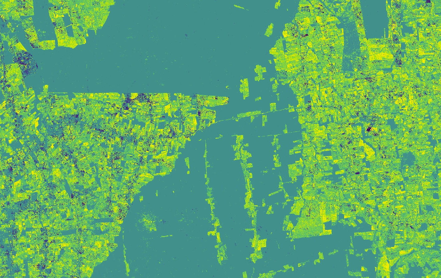
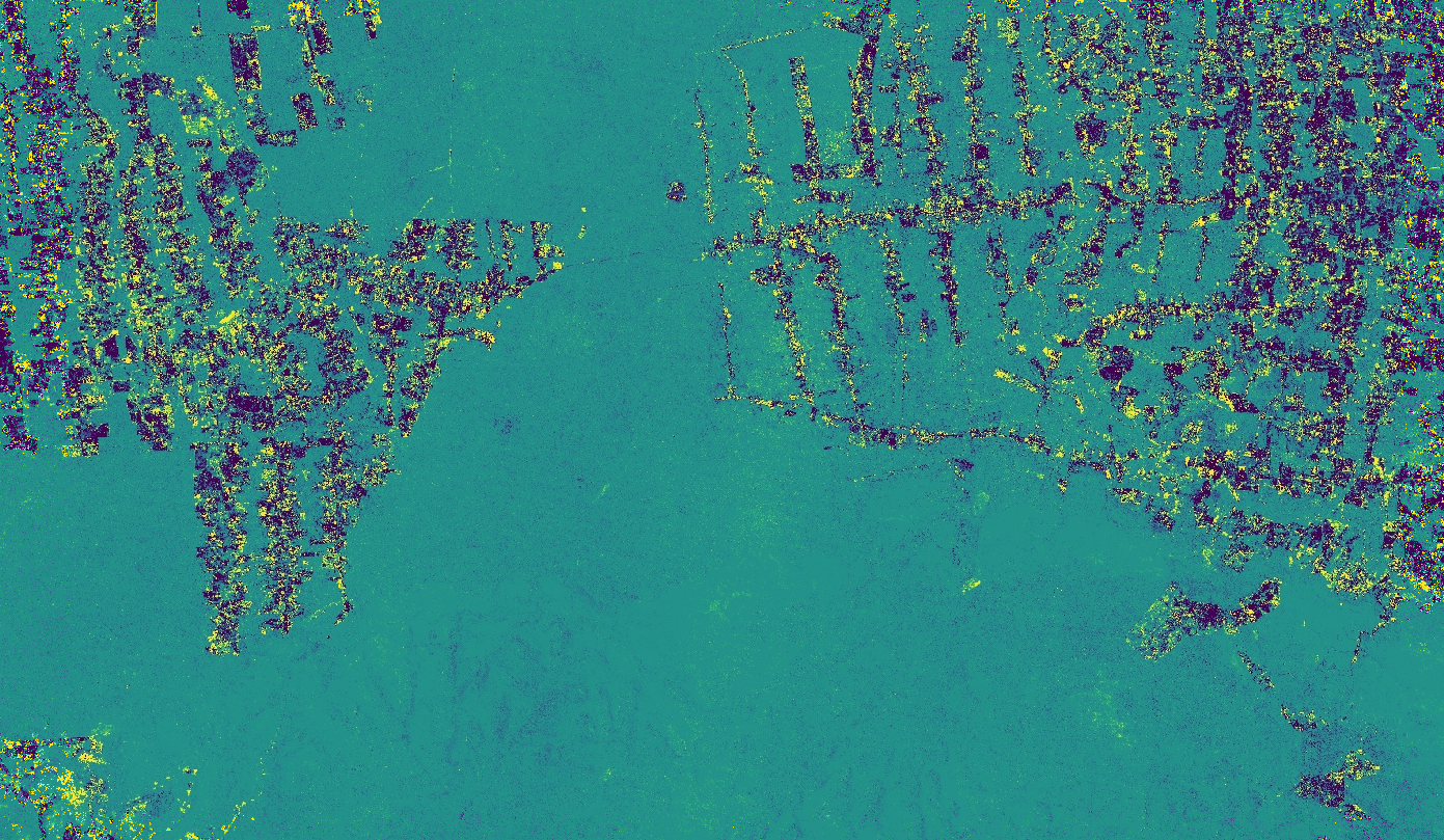
For places with many changes, visualizing the first or last time when a break was recorded can be helpful to understand the change dynamics happening in the landscape. Paste the code below in the same script:

Here we use arrayMask to keep only the change dates that meet our condition, by using the mask we created previously. We use the function arrayPad to fill or “pad” those pixels that did not experience any change and therefore have no value in the tBreak band. Then we select either the first or last values in the array, and we convert the image from a one-dimensional array to a regular image, in order to apply a visualization to it, using a custom palette. The results should look like Fig. F4.7.2.

Finally, we can use the magnitude bands to visualize where and when the largest changes as recorded by CCDC have occurred, during our selected time period. We are going to use the magnitude of change in the SWIR1 band, masking it and padding it in the same way we did before. Paste this code in your script:

We first take the absolute value because the magnitudes can be positive or negative, depending on the direction of the change and the band used. For example, a positive value in the SWIR1 may show a forest loss event, where surface reflectance goes from low to higher values. Brighter values in Fig. 4.7.3 represent events of that type. Conversely, a flooding event would have a negative value, due to the corresponding drop in reflectance. Once we find the maximum absolute value, we find its position on the array and then use that index to extract the original magnitude value, as well as the time when that break occurred.

Code Checkpoint F47c. The book’s repository contains a script that shows what your code should look like at this point.

Question 2. Compare the “first change” and “last change” layers with the layer showing the timing of the maximum magnitude of change. Use the Inspector to check the values for specific pixels if necessary. What does the timing of the layers tell you about the change processes happening in the area?

Question 3. Looking at the “max magnitude of change” layer, find places showing the largest and the smallest values. What type of changes do you think are happening in each of those places?

Section 4. Extracting Coefficients Manually

In addition to the change information generated by the CCDC algorithm, we can use the coefficients of the time segments for multiple purposes, like land cover classification. Each time segment can be described as a harmonic function with an intercept, slope, and three pairs of sine and cosine terms that allow the time segments to represent seasonality occurring at different temporal scales. These coefficients, as well as the root-mean-square error (RMSE) obtained by comparing each predicted and actual Landsat value, are produced when the CCDC algorithm is run. The following example will show you how to retrieve the intercept coefficient for a segment intersecting a specific date. In a new script, paste the code below:

Check the Console and expand the bands section in the printed image information. We will be using the tStart, tEnd, and SWIR1_coefs bands, which are array images containing the date when the time segments start, date time segments end, and the coefficients for each of those segments for the SWIR1 band. Run the code above and switch the map to Satellite mode. Using the Inspector, click anywhere on the images, noticing the number of dates printed and their values for multiple clicked pixels. You will notice that for places with stable forest cover, there is usually one value for tStart and one for tEnd. This means that for those more stable places, only one time segment was fit by CCDC. On the other hand, for places with visible transformation in the basemap, the number of dates is usually two or three, meaning that the algorithm fitted two or three time segments, respectively. To simplify the processing of the data, we can select a single segment to extract its coefficients. Paste the code below and re-run the script:

In the code above, we set a time of interest, in this case the middle of 2005, and then we find the segments that meet the condition of starting before and ending after that date. Using the Inspector again, click on different locations and verify the outputs. The segment that meets the condition will have a value of 1, and the other segments will have a value of 0. We can use this information to select the coefficients for that segment, using the code below:

In the piece of code above, we first select the array image with the coefficients for the SWIR1 band. Then, using the layer that we created before, we find the position where the condition is true, and use that to extract the coefficients only for that segment. Once again, you can verify that using the Inspector tab.

Finally, what we have now is the full set of coefficients for the segment that intersects the midpoint of 2005. The coefficients are in the following order: intercept, slope, cosine 1, sine 1, cosine 2, sine 2, cosine 3, and sine 3. For this exercise we will extract the intercept coefficient (Fig. 4.7.4), which is the first element in the array, using the code below:

Since we run the CCDC algorithm on Landsat surface reflectance images, intercept values should represent the average reflectance of a segment. However, if you click on the image, you will see that the values are outside of the 0–1 range. This is because the intercept is calculated by the CCDC algorithm for the origin (e.g., time 0), and not for the year we requested. In order to retrieve the adjusted intercept, as well as other coefficients, we will use a different approach.

Code Checkpoint F47d. The book’s repository contains a script that shows what your code should look like at this point.

Section 5. Extracting Coefficients Using External Functions

The code we generated in the previous section allowed us to extract a single coefficient for a single date. However, we typically want to extract a set of multiple coefficients and bands that we can use as inputs to other workflows, such as classification. To simplify that process, we will use the same function library that we saw in Sect. 2. In this section we will extract and visualize different coefficients for a single date and produce an RGB image using the intercept coefficients for multiple spectral bands for the same date. The first step involves determining the date of interest and converting the CCDC results from array images to regular multiband images for easier manipulation and faster display. In a new script, copy the code below:

In the code above we define the date of interest (2005-09-25) and convert it to the date format in which we ran CCDC, which corresponds to fractional years. After that, we specify the band that we used as inputs for the CCDC algorithm. Finally, we specify the names we will assign to the time segments, with the list length indicating the maximum number of time segments to retrieve per pixel. This step is done because the results generated by CCDC are stored as variable-length arrays. For example, a pixel where there are no breaks detected will have one time segment, but another pixel where a single break was detected may have one or two segments, depending on when the break occurred. Requesting a pre-defined maximum number of segments ensures that the structure of the multi-band image is known, and greatly facilitates its manipulation and display. Once we have set these variables, we call a function that converts the result into an image with several bands representing the combination of segments requested, input bands, and coefficients. You can see the image structure in the Console.

Finally, to extract a subset of coefficients for the desired bands, we can use a function in the imported library, called getMultiCoefs. This function expects the following ordered parameters:

• The CCDC results in the multiband format we just generated in the step above.
• The date for which we want to extract the coefficients, in the format in which the CCDC results were run (fractional years in our case).
• List of the bands to retrieve (i.e., spectral bands).
• List of coefficients to retrieve, defined as follows: INTP (intercept), SLP (slope), COS, SIN,COS32, SIN2, COS3, SIN3, and RMSE.
• A Boolean flag of true or false, indicating whether we want the intercepts to be calculated for the input date, instead of being calculated at the origin. If true, SLP must be included in the list of coefficients to retrieve.
• List of segment names, as used to create the multiband image in the prior step.
• Behavior to apply if there is no time segment for the requested date: normal will retrieve a value only if the date intersects a segment;        before or after will use the value of the segment immediately before or after the requested date, if no segment intersects the date directly.

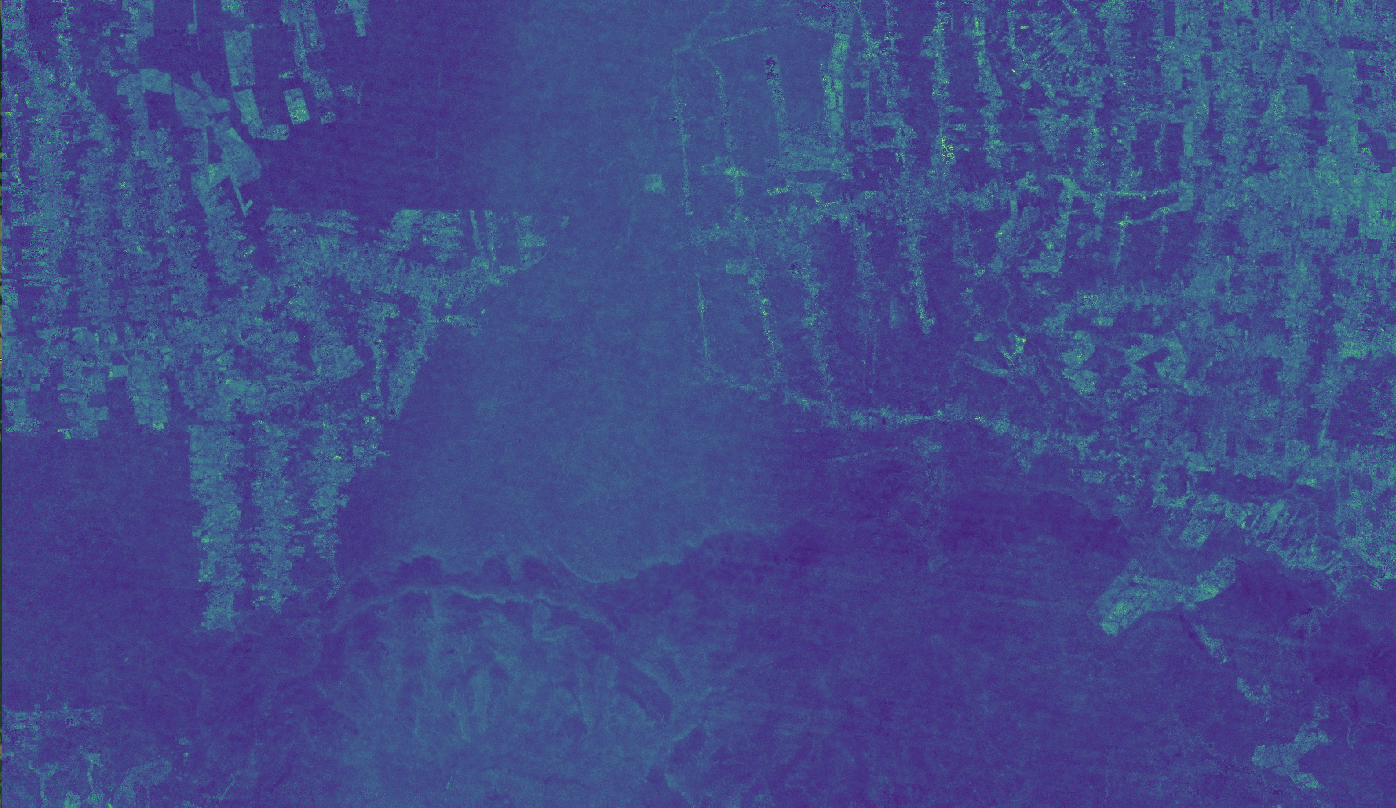
The slope and RMSE images are shown in Fig. 4.7.5. For the slopes, high positive values are bright, while large negative values are very dark. Most of the remaining forest is stable and has a slope close to zero, while areas that have experienced transformation and show agricultural activity tend to have positive slopes in the RED band, appearing bright in the image. Similarly, for the RMSE image, stable forests present more predictable time series of surface reflectance that are captured more faithfully by the time segments, and therefore present lower RMSE values, appearing darker in the image. Agricultural areas present noisier time series that are more challenging to model, and result in higher RMSE values, appearing brighter.

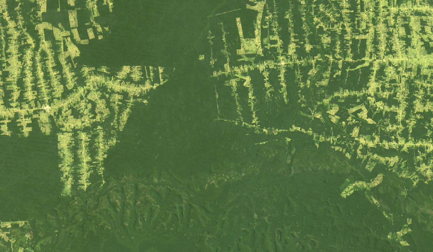
Finally, the RGB image we created is shown in Fig. 4.7.6. The intercepts are calculated for the middle point of the time segment intercepting the date we requested, representing the average reflectance for the span of the selected segment. In that sense, when shown together as an RGB image, they are similar to a composite image for the selected date, with the advantage of always being cloud-free.

Code Checkpoint F47e. The book’s repository contains a script that shows what your code should look like at this point.

Synthesis

Assignment 1. Use the time series from the first section of this chapter to explore the time series and time segments produced by CCDC in many locations around the world. Compare places with different land cover types, and places with more stable dynamics (e.g., lakes, primary forests) vs. highly dynamic places (e.g., agricultural lands, construction sites). Pay attention to the variability in data density across continents and latitudes, and the effect that data density has on the appearance of the time segments. Use different spectral bands and indices and notice how they capture the temporal dynamics you are observing.

Assignment 2. Pick three periods within the temporal study period of the CCDC results we used earlier: one near to the start, another in the middle, and the third close to the end. For each period, visualize the maximum change magnitude. Compare the spatial patterns between periods, and reflect on the types of disturbances that might be happening at each stage.

Assignment 3. Select the intercept coefficients of the middle date of each of the periods you chose in the previous assignment. For each of those dates, load an RGB image with the band combination of your choosing (or simply use the Red, Green and Blue intercepts to obtain true-color images). Using the Inspector tab, compare the values across images in places with subtle and large differences between them, as well as in areas that do not change. What do the values tell you in terms of the benefits of using CCDC to study changes in a landscape?

Conclusion

This chapter provided a guide for the interpretation of the results from the CCDC algorithm for studying deforestation in the Amazon. Consider the advantages of such an analysis compared to traditional approaches to change detection, which are typically based on the comparison of two or a few images collected over the same area. For example, with time-series analysis, we can study trends and subtle processes such as vegetation recovery or degradation, determine the timing of land-surface events, and move away from retrospective analyses to monitoring in near-real time. Through the use of all available clear observations, CCDC can detect intra-annual breaks and capture seasonal patterns, although at the expense of increased computational requirements and complexity, unlike faster and easier to interpret methods based on annual composites, such as LandTrendr (Chap. F4.5). We expect to see more applications that make use of multiple change detection approaches (also known as “Ensemble” approaches), and multisensor analyses in which data from different satellites are fused (radar and optical, for example) for higher data density.

Feedback

To review this chapter and make suggestions or note any problems, please go now to bit.ly/EEFA-review. You can find summary statistics from past reviews at bit.ly/EEFA-reviews-stats.

References

Cloud-Based Remote Sensing with Google Earth Engine. (n.d.). CLOUD-BASED REMOTE SENSING WITH GOOGLE EARTH ENGINE. https://www.eefabook.org/

Cloud-Based Remote Sensing with Google Earth Engine. (2024). In Springer eBooks. https://doi.org/10.1007/978-3-031-26588-4

Arévalo P, Bullock EL, Woodcock CE, Olofsson P (2020) A suite of tools for continuous land change monitoring in Google Earth Engine. Front Clim 2. https://doi.org/10.3389/fclim.2020.576740

Box GEP, Jenkins GM, Reinsel GC (1994) Time Series Analysis: Forecasting and Control. Prentice Hall

Gorelick N, Hancher M, Dixon M, et al (2017) Google Earth Engine: Planetary-scale geospatial analysis for everyone. Remote Sens Environ 202:18–27. https://doi.org/10.1016/j.rse.2017.06.031

Kennedy RE, Andréfouët S, Cohen WB, et al (2014) Bringing an ecological view of change to Landsat-based remote sensing. Front Ecol Environ 12:339–346. https://doi.org/10.1890/130066

Woodcock CE, Loveland TR, Herold M, Bauer ME (2020) Transitioning from change detection to monitoring with remote sensing: A paradigm shift. Remote Sens Environ 238:111558. https://doi.org/10.1016/j.rse.2019.111558

Zhu Z, Woodcock CE (2014) Continuous change detection and classification of land cover using all available Landsat data. Remote Sens Environ 144:152–171. https://doi.org/10.1016/j.rse.2014.01.011