Cloud-Based Remote Sensing with Google Earth Engine
Fundamentals and Applications

Part F2: Interpreting Images
Now that you know how images are viewed and what kinds of images exist in Earth Engine, how do we manipulate them? To gain the skills of interpreting images, you’ll work with bands, combining values to form indices and masking unwanted pixels. Then, you’ll learn some of the techniques available in Earth Engine for classifying images and interpreting the results.
Chapter F2.0: Image Manipulation: Bands, Arithmetic, Thresholds, and Masks
Authors
Karen Dyson, Andréa Puzzi Nicolau, David Saah, and Nicholas Clinton
Overview
Once images have been identified in Earth Engine, they can be viewed in a wide array of band combinations for targeted purposes. For users who are already versed in remote sensing concepts, this chapter shows how to do familiar tasks on this platform; for those who are entirely new to such concepts, it introduces the idea of band combinations.
Learning Outcomes
- Understanding what spectral indices are and why they are useful.
- Being introduced to a range of example spectral indices used for a variety of purposes.
Assumes you know how to:
- Import images and image collections, filter, and visualize (Part F1).
Github Code link for all tutorials
This code base is collection of codes that are freely available from different authors for google earth engine.
Introduction to Theory
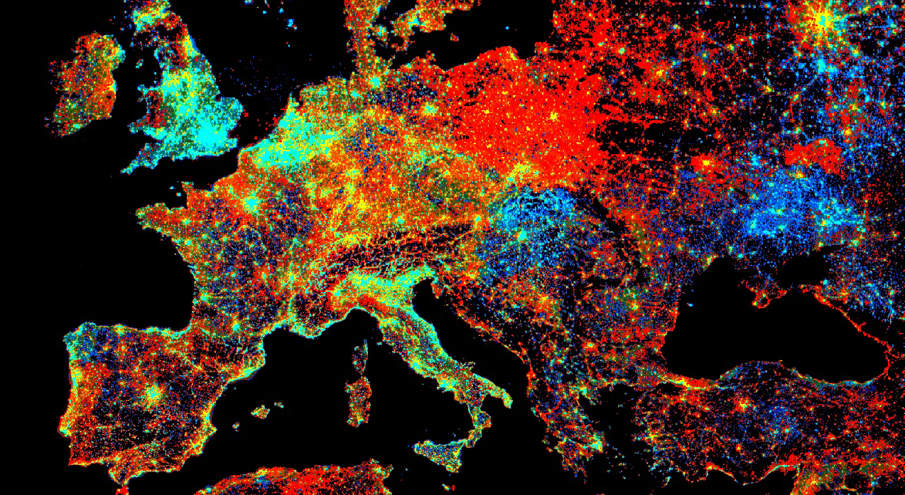
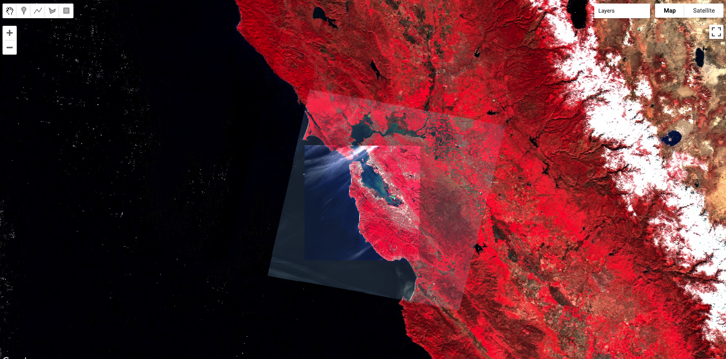
Spectral indices are based on the fact that different objects and land covers on the Earth’s surface reflect different amounts of light from the Sun at different wavelengths. In the visible part of the spectrum, for example, a healthy green plant reflects a large amount of green light while absorbing blue and red light—which is why it appears green to our eyes. Light also arrives from the Sun at wavelengths outside what the human eye can see, and there are large differences in reflectances between living and nonliving land covers, and between different types of vegetation, both in the visible and outside the visible wavelengths. We visualized this earlier, in Chaps. F1.1 and F1.3 when we mapped color-infrared images (Fig. F2.0.1).
Fig. F2.0.1 Mapped color-IR images from multiple satellite sensors that we mapped in Chap. F1.3. The near infrared spectrum is mapped as red, showing where there are high amounts of healthy vegetation. |
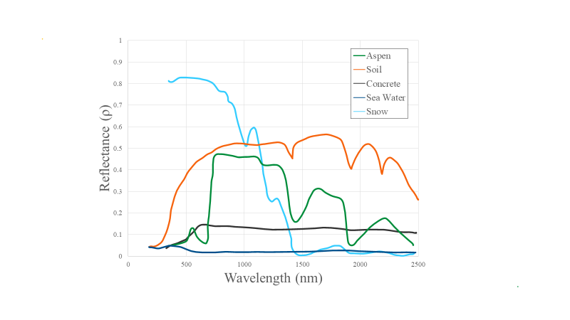
If we graph the amount of light (reflectance) at different wavelengths that an object or land cover reflects, we can visualize this more easily (Fig. F2.0.2). For example, look at the reflectance curves for soil and water in the graph below. Soil and water both have relatively low reflectance at wavelengths around 300 nm (ultraviolet and violet light). Conversely, at wavelengths above 700 nm (red and infrared light) soil has relatively high reflectance, while water has very low reflectance. Vegetation, meanwhile, generally reflects large amounts of near infrared light, relative to other land covers.
Fig. F2.0.2 A graph of the amount of reflectance for different objects on the Earth’s surface at different wavelengths in the visible and infrared portions of the electromagnetic spectrum. 1 micrometer (µm)=1,000 nanometers (nm). |
Spectral indices use math to express how objects reflect light across multiple portions of the spectrum as a single number. Indices combine multiple bands, often with simple operations of subtraction and division, to create a single value across an image that is intended to help to distinguish particular land uses or land covers of interest. Using Fig. F2.0.2, you can imagine which wavelengths might be the most informative for distinguishing among a variety of land covers. We will explore a variety of calculations made from combinations of bands in the following sections.
Indices derived from satellite imagery are used as the basis of many remote-sensing analyses. Indices have been used in thousands of applications, from detecting anthropogenic deforestation to examining crop health. For example, the growth of economically important crops such as wheat and cotton can be monitored throughout the growing season: Bare soil reflects more red wavelengths, whereas growing crops reflect more of the near-infrared (NIR) wavelengths. Thus, calculating a ratio of these two bands can help monitor how well crops are growing (Jackson and Huete 1991).
Practicum
Section 1. Band Arithmetic in Earth Engine
If you have not already done so, be sure to add the book’s code repository to the Code Editor by entering https://code.earthengine.google.com/?accept_repo=projects/gee-edu/book into your browser. The book’s scripts will then be available in the script manager panel. If you have trouble finding the repo, you can visit this link for help.
Many indices can be calculated using band arithmetic in Earth Engine. Band arithmetic is the process of adding, subtracting, multiplying, or dividing two or more bands from an image. Here we’ll first do this manually, and then show you some more efficient ways to perform band arithmetic in Earth Engine.
Arithmetic Calculation of NDVI
The red and near-infrared bands provide a lot of information about vegetation due to vegetation’s high reflectance in these wavelengths. Take a look at Fig. F2.0.2 and note, in particular, that vegetation curves (graphed in green) have relatively high reflectance in the NIR range (approximately 750–900 nm). Also note that vegetation has low reflectance in the red range (approximately 630–690 nm), where sunlight is absorbed by chlorophyll. This suggests that if the red and near-infrared bands could be combined, they would provide substantial information about vegetation.
Soon after the launch of Landsat 1 in 1972, analysts worked to devise a robust single value that would convey the health of vegetation along a scale of −1 to 1. This yielded the NDVI, using the formula:
 (F2.0.1)
where NIR and red refer to the brightness of each of those two bands. As seen in Chaps. F1.1 and F1.2, this brightness might be conveyed in units of reflectance, radiance, or digital number (DN); the NDVI is intended to give nearly equivalent values across platforms that use these wavelengths. The general form of this equation is called a “normalized difference”—the numerator is the “difference” and the denominator “normalizes” the value. Outputs for NDVI vary between −1 and 1. High amounts of green vegetation have values around 0.8–0.9. Absence of green leaves gives values near 0, and water gives values near −1.
To compute the NDVI, we will introduce Earth Engine’s implementation of band arithmetic. Cloud-based band arithmetic is one of the most powerful aspects of Earth Engine, because the platform’s computers are optimized for this type of heavy processing. Arithmetic on bands can be done even at planetary scale very quickly—an idea that was out of reach before the advent of cloud-based remote sensing. Earth Engine automatically partitions calculations across a large number of computers as needed, and assembles the answer for display.
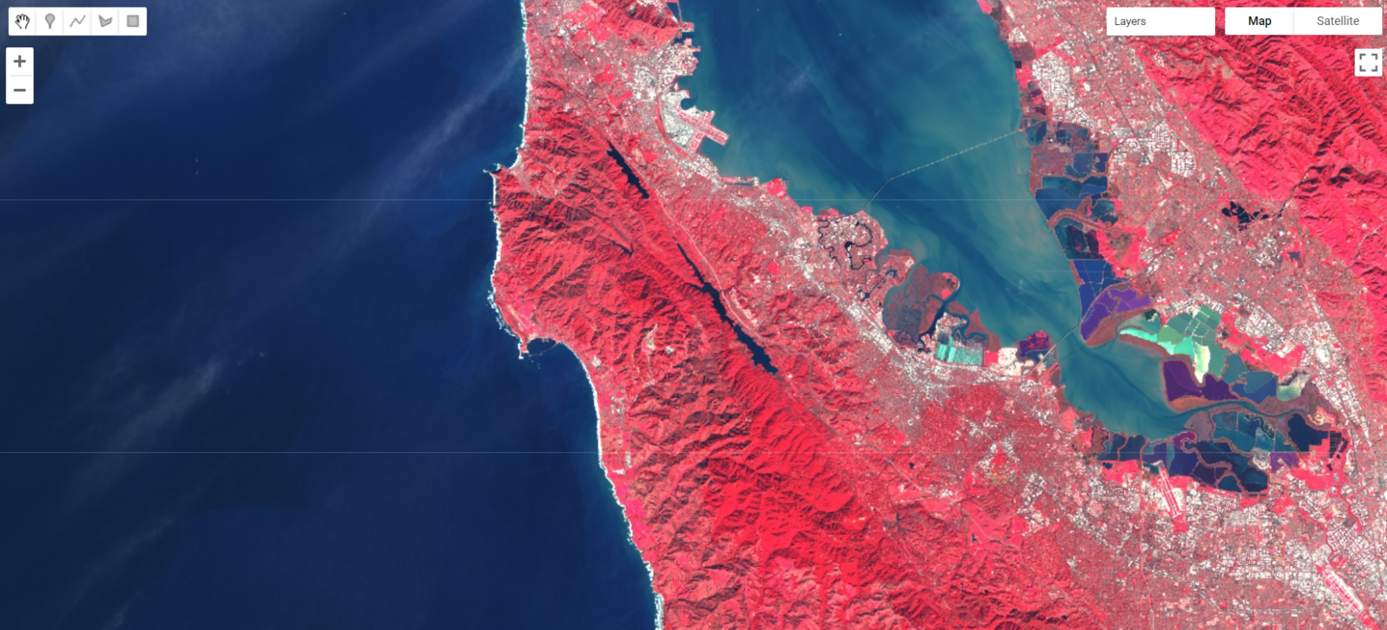
As an example, let’s examine an image of San Francisco (Fig. F2.0.3).
///// |
Fig. F2.0.3 False color Sentinel-2 imagery of San Francisco and surroundings |
The simplest mathematical operations in Earth Engine are the add, subtract, multiply, and divide methods. Let’s select the near-infrared and red bands and use these operations to calculate NDVI for our image.
// Extract the near infrared and red bands. |
Examine the resulting index, using the Inspector to pick out pixel values in areas of vegetation and non-vegetation if desired.
Fig. F2.0.4 NDVI calculated using Sentinel-2. Remember that outputs for NDVI vary between −1 and 1. High amounts of green vegetation have values around 0.8–0.9. Absence of green leaves gives values near 0, and water gives values near −1. |

Using these simple arithmetic tools, you can build almost any index, or develop and visualize your own. Earth Engine allows you to quickly and easily calculate and display the index across a large area.
Single-Operation Computation of Normalized Difference for NDVI
Normalized differences like NDVI are so common in remote sensing that Earth Engine provides the ability to do that particular sequence of subtraction, addition, and division in a single step, using the normalizedDifference method. This method takes an input image, along with bands you specify, and creates a normalized difference of those two bands. The NDVI computation previously created with band arithmetic can be replaced with one line of code:
// Now use the built-in normalizedDifference function to achieve the same outcome. |
Note that the order in which you provide the two bands to normalizedDifference is important. We use B8, the near-infrared band, as the first parameter, and the red band B4 as the second. If your two computations of NDVI do not look identical when drawn to the screen, check to make sure that the order you have for the NIR and red bands is correct.
Using Normalized Difference for NDWI
As mentioned, the normalized difference approach is used for many different indices. Let’s apply the same normalizedDifference method to another index.
The Normalized Difference Water Index (NDWI) was developed by Gao (1996) as an index of vegetation water content. The index is sensitive to changes in the liquid content of vegetation canopies. This means that the index can be used, for example, to detect vegetation experiencing drought conditions or differentiate crop irrigation levels. In dry areas, crops that are irrigated can be differentiated from natural vegetation. It is also sometimes called the Normalized Difference Moisture Index (NDMI). NDWI is formulated as follows:
 (F2.0.2)
where NIR is near-infrared, centered near 860 nm (0.86 μm), and SWIR is short-wave infrared, centered near 1,240 nm (1.24 μm).
Compute and display NDWI in Earth Engine using the normalizedDifference method. Remember that for Sentinel-2, B8 is the NIR band and B11 is the SWIR band (refer to Chaps. F1.1 and F1.3 to find information about imagery bands).
// Use normalizedDifference to calculate NDWI |
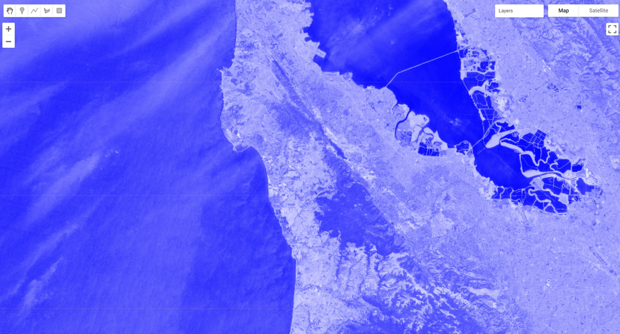
Examine the areas of the map that NDVI identified as having a lot of vegetation. Notice which are more blue. This is vegetation that has higher water content.
Fig. F2.0.5 NDWI displayed for Sentinel-2 over San Francisco |
Code Checkpoint F20a. The book’s repository contains a script that shows what your code should look like at this point.
Section 2. Thresholding, Masking, and Remapping Images
The previous section in this chapter discussed how to use band arithmetic to manipulate images. Those methods created new continuous values by combining bands within an image. This section uses logical operators to categorize band or index values to create a categorized image.
Implementing a Threshold
Implementing a threshold uses a number (the threshold value) and logical operators to help us partition the variability of images into categories. For example, recall our map of NDVI. High amounts of vegetation have NDVI values near 1 and non-vegetated areas are near 0. If we want to see what areas of the map have vegetation, we can use a threshold to generalize the NDVI value in each pixel as being either “no vegetation” or “vegetation”. That is a substantial simplification, to be sure, but can help us to better comprehend the rich variation on the Earth’s surface. This type of categorization may be useful if, for example, we want to look at the proportion of a city that is vegetated. Let’s create a Sentinel-2 map of NDVI near Seattle, Washington, USA. Enter the code below in a new script.
// Create an NDVI image using Sentinel 2. |
Fig. F2.0.6 NDVI image of Sentinel-2 imagery over Seattle, Washington, USA |
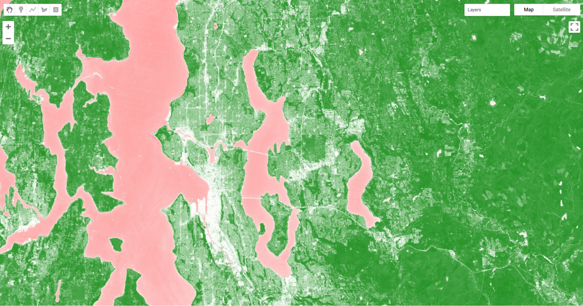
Inspect the image. We can see that vegetated areas are darker green while non-vegetated locations are white and water is pink. If we use the Inspector to query our image, we can see that parks and other forested areas have an NDVI over about 0.5. Thus, it would make sense to define areas with NDVI values greater than 0.5 as forested, and those below that threshold as not forested.
Now let’s define that value as a threshold and use it to threshold our vegetated areas.
// Implement a threshold. |
The gt method is from the family of Boolean operators—that is, gt is a function that performs a test in each pixel and returns the value 1 if the test evaluates to true, and 0 otherwise. Here, for every pixel in the image, it tests whether the NDVI value is greater than 0.5. When this condition is met, the layer seaVeg gets the value 1. When the condition is false, it receives the value 0.
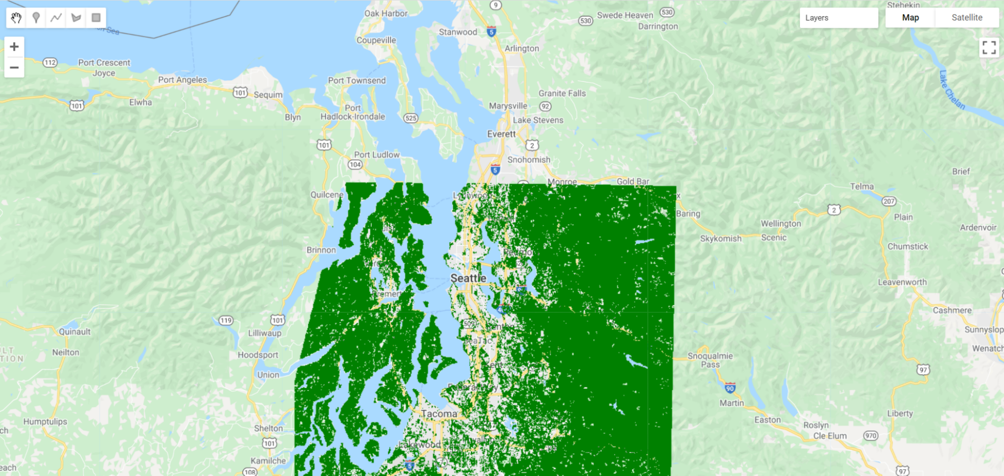
Fig. F2.0.7 Thresholded forest and non-forest image based on NDVI for Seattle, Washington, USA |
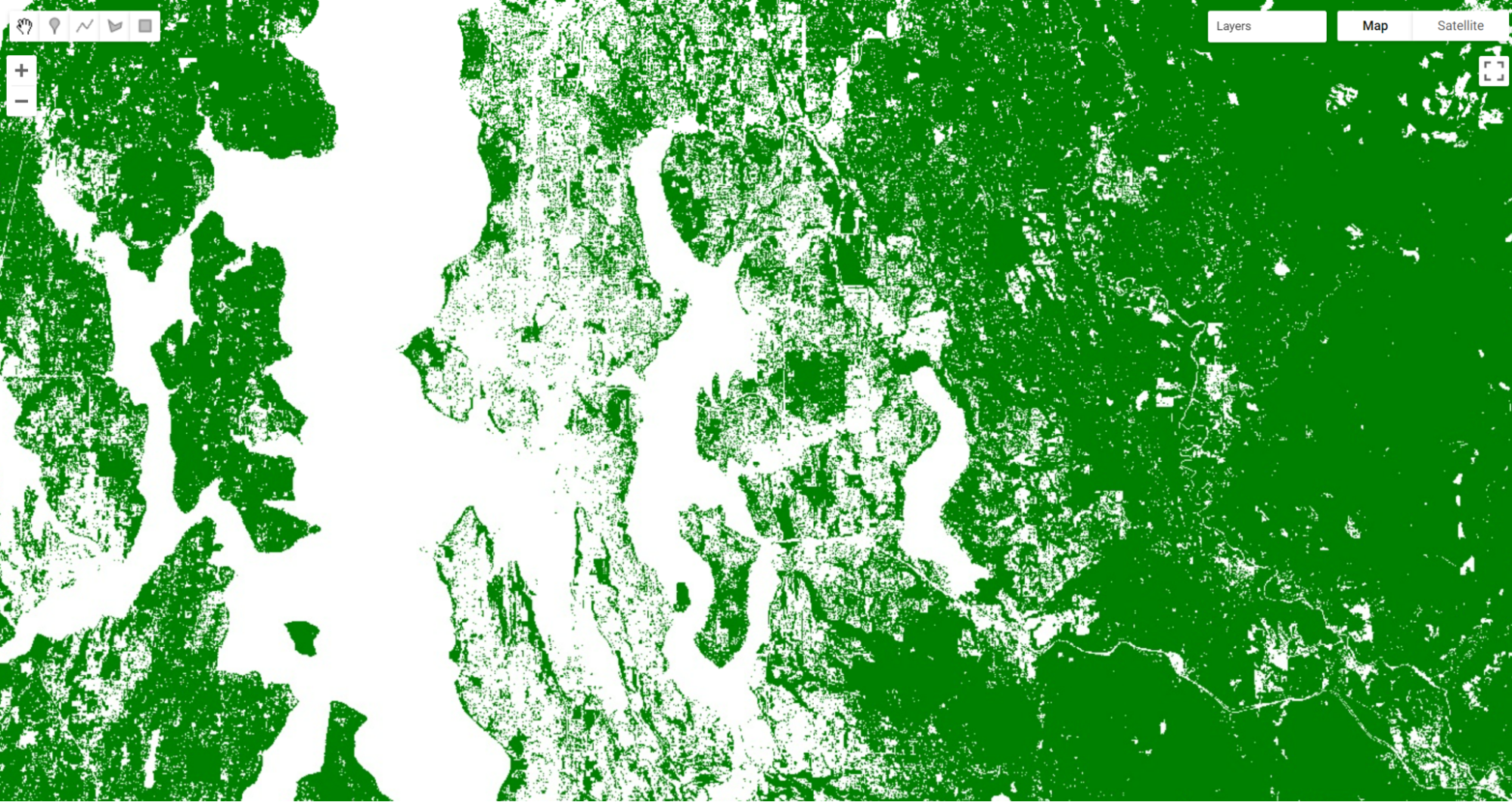
Use the Inspector tool to explore this new layer. If you click on a green location, that NDVI should be greater than 0.5. If you click on a white pixel, the NDVI value should be equal to or less than 0.5.
Other operators in this Boolean family include less than (lt), less than or equal to (lte), equal to (eq), not equal to (neq), and greater than or equal to (gte) and more.
Building Complex Categorizations with .where
A binary map classifying NDVI is very useful. However, there are situations where you may want to split your image into more than two bins. Earth Engine provides a tool, the where method, that conditionally evaluates to true or false within each pixel depending on the outcome of a test. This is analogous to an if statement seen commonly in other languages. However, to perform this logic when programming for Earth Engine, we avoid using the JavaScript if statement. Importantly, JavaScript if commands are not calculated on Google’s servers, and can create serious problems when running your code—in effect, the servers try to ship all of the information to be executed to your own computer’s browser, which is very underequipped for such enormous tasks. Instead, we use the where clause for conditional logic.
Suppose instead of just splitting the forested areas from the non-forested areas in our NDVI, we want to split the image into likely water, non-forested, and forested areas. We can use where and thresholds of -0.1 and 0.5. We will start by creating an image using ee.Image. We then clip the new image so that it covers the same area as our seaNDVI layer.
// Implement .where. |
There are a few interesting things to note about this code that you may not have seen before. First, we’re not defining a new variable for each where call. As a result, we can perform many where calls without creating a new variable each time and needing to keep track of them. Second, when we created the starting image, we set the value to 1. This means that we could easily set the bottom and top values with one where clause each. Finally, while we did not do it here, we can combine multiple where clauses using and and or. For example, we could identify pixels with an intermediate level of NDVI using seaNDVI.gte(-0.1).and(seaNDVI.lt(0.5)).
Fig. F2.0.8 Thresholded water, forest, and non-forest image based on NDVI for Seattle, Washington, USA. |

Masking Specific Values in an Image
Masking an image is a technique that removes specific areas of an image—those covered by the mask—from being displayed or analyzed. Earth Engine allows you to both view the current mask and update the mask.
// Implement masking. |
Fig. F2.0.9 The existing mask for the seaVeg layer we created previously |
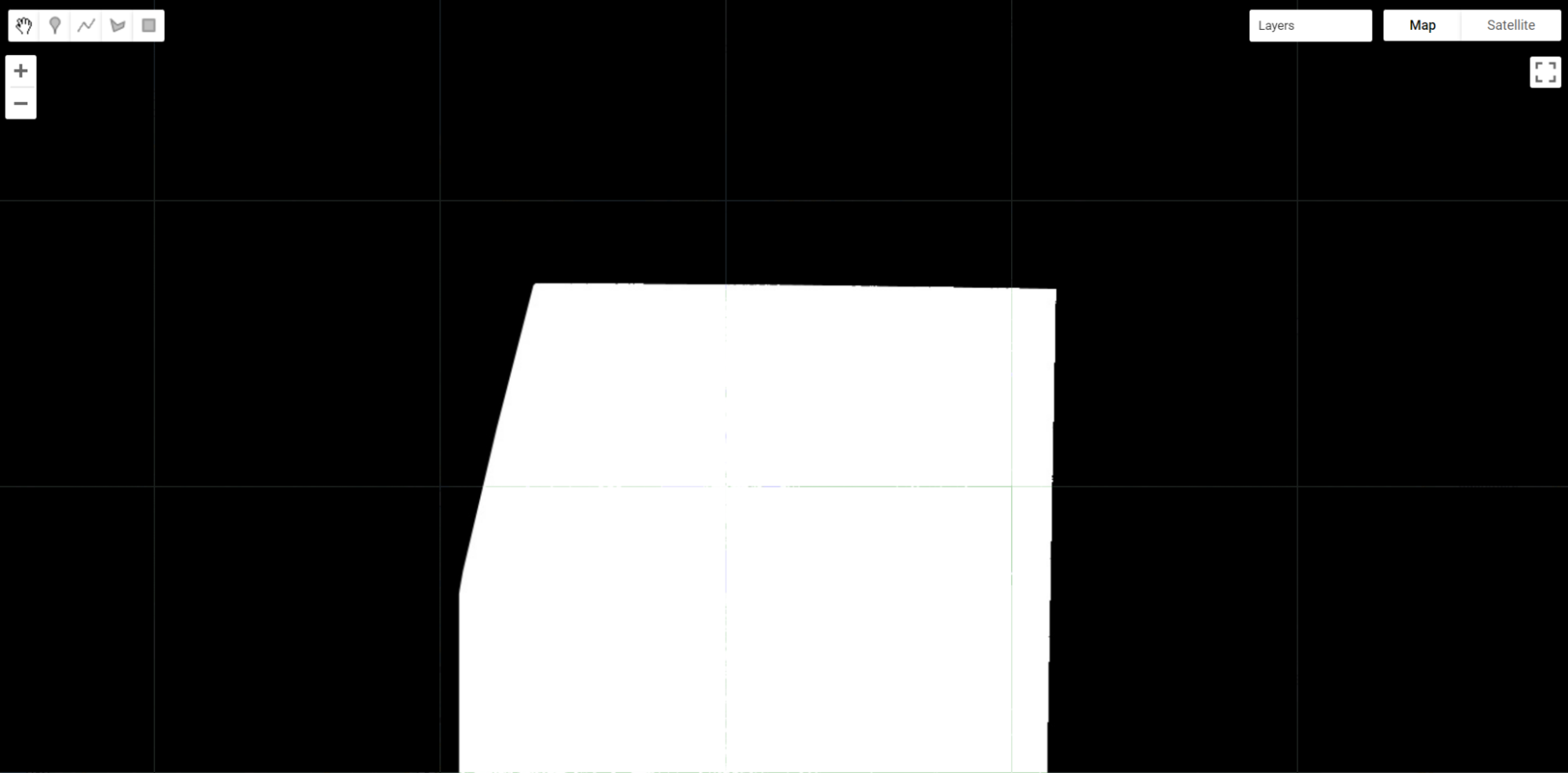
You can use the Inspector to see that the black area is masked and the white area has a constant value of 1. This means that data values are mapped and available for analysis within the white area only.
Now suppose we only want to display and conduct analyses in the forested areas. Let’s mask out the non-forested areas from our image. First, we create a binary mask using the equals (eq) method.
// Create a binary mask of non-forest. |
In making a mask, you set the values you want to see and analyze to be a number greater than 0. The idea is to set unwanted values to get the value of 0. Pixels that had 0 values become masked out (in practice, they do not appear on the screen at all) once we use the updateMask method to add these values to the existing mask.
// Update the seaVeg mask with the non-forest mask. |
Turn off all of the other layers. You can see how the maskedVeg layer now has masked out all non-forested areas.
Fig. F2.0.10 An updated mask now displays only the forested areas. Non-forested areas are masked out and transparent. |
Map the updated mask for the layer and you can see why this is.
// Map the updated mask |
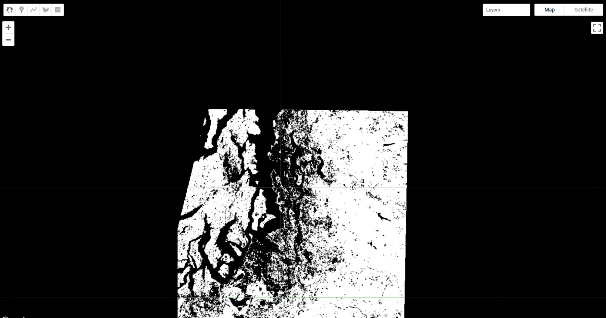
Fig. F2.0.11 The updated mask. Areas of non-forest are now masked out as well (black areas of the image). |
Remapping Values in an Image
Remapping takes specific values in an image and assigns them a different value. This is particularly useful for categorical datasets, including those you read about in Chap. F1.2 and those we have created earlier in this chapter.
Let’s use the remap method to change the values for our seaWhere layer. Note that since we’re changing the middle value to be the largest, we’ll need to adjust our palette as well.
// Implement remapping. |
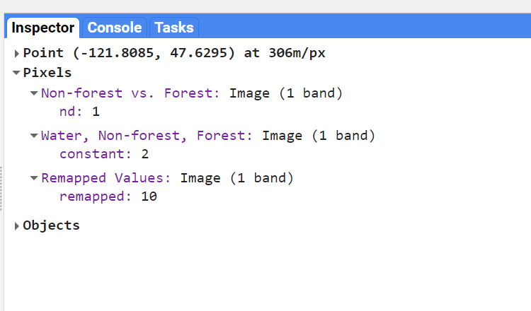
Use the inspector to compare values between our original seaWhere (displayed as Water, Non-Forest, Forest) and the seaRemap, marked as “Remapped Values.” Click on a forested area and you should see that the Remapped Values should be 10, instead of 2 (Fig. F2.0.12).
Fig. F2.0.12 For forested areas, the remapped layer has a value of 10, compared with the original layer, which has a value of 2. You may have more layers in your Inspector. |
Code Checkpoint F20b. The book’s repository contains a script that shows what your code should look like at this point.
Synthesis
Assignment 1. In addition to vegetation indices and other land cover indices, you can use properties of different soil types to create geological indices. The Clay Minerals Ratio (CMR) is one of these. This index highlights soils containing clay and alunite, which absorb radiation in the SWIR portion (2.0–2.3 μm) of the spectrum.

SWIR 1 should be in the 1.55–1.75 µm range, and SWIR 2 should be in the 2.08–2.35 µm range. Calculate and display CMR at the following point: ee.Geometry.Point(-100.543, 33.456). Don’t forget to use Map.centerObject.
We’ve selected an area of Texas known for its clay soils. Compare this with an area without clay soils (for example, try an area around Seattle or Tacoma, Washington, USA). Note that this index will also pick up roads and other paved areas.
Assignment 2. Calculate the Iron Oxide Ratio, which can be used to detect hydrothermally altered rocks (e.g., from volcanoes) that contain iron-bearing sulfides which have been oxidized (Segal, 1982).
Here’s the formula:

Red should be the 0.63–0.69 µm spectral range and Blue the 0.45–0.52 µm. Using Landsat 8, you can also find an interesting area to map by considering where these types of rocks might occur.
Assignment 3. Calculate the Normalized Difference Built-Up Index (NDBI) for the sfoImage used in this chapter.
The NDBI was developed by Zha et al. (2003) to aid in differentiating urban areas (e.g., densely clustered buildings and roads) from other land cover types. The index exploits the fact that urban areas, which generally have a great deal of impervious surface cover, reflect SWIR very strongly. If you like, refer back to Fig. F2.0.2.
The formula is:

Using what we know about Sentinel-2 bands, compute NDBI and display it.
Bonus: Note that NDBI is the negative of NDWI computed earlier. We can prove this by using the JavaScript reverse method to reverse the palette used for NDWI in Earth Engine. This method reverses the order of items in the JavaScript list. Create a new palette for NDBI using the reverse method and display the map. As a hint, here is code to use the reverse method.
var barePalette=waterPalette.reverse(); |
Conclusion
In this chapter, you learned how to select multiple bands from an image and calculate indices. You also learned about thresholding values in an image, slicing them into multiple categories using thresholds. It is also possible to work with one set of class numbers and remap them quickly to another set. Using these techniques, you have some of the basic tools of image manipulation. In subsequent chapters you will encounter more complex and specialized image manipulation techniques, including pixel-based image transformations (Chap. F3.1), neighborhood-based image transformations (Chap. F3.2), and object-based image analysis (Chap. F3.3).
Feedback
To review this chapter and make suggestions or note any problems, please go now to bit.ly/EEFA-review. You can find summary statistics from past reviews at bit.ly/EEFA-reviews-stats.
References
Cloud-Based Remote Sensing with Google Earth Engine. (n.d.). CLOUD-BASED REMOTE SENSING WITH GOOGLE EARTH ENGINE. https://www.eefabook.org/
Cloud-Based Remote Sensing with Google Earth Engine. (2024). In Springer eBooks. https://doi.org/10.1007/978-3-031-26588-4
Baig MHA, Zhang L, Shuai T, Tong Q (2014) Derivation of a tasselled cap transformation based on Landsat 8 at-satellite reflectance. Remote Sens Lett 5:423–431. https://doi.org/10.1080/2150704X.2014.915434
Crist EP (1985) A TM tasseled cap equivalent transformation for reflectance factor data. Remote Sens Environ 17:301–306. https://doi.org/10.1016/0034-4257(85)90102-6
Drury SA (1987) Image interpretation in geology. Geocarto Int 2:48. https://doi.org/10.1080/10106048709354098
Gao BC (1996) NDWI - A normalized difference water index for remote sensing of vegetation liquid water from space. Remote Sens Environ 58:257–266. https://doi.org/10.1016/S0034-4257(96)00067-3
Huang C, Wylie B, Yang L, et al (2002) Derivation of a tasselled cap transformation based on Landsat 7 at-satellite reflectance. Int J Remote Sens 23:1741–1748. https://doi.org/10.1080/01431160110106113
Jackson RD, Huete AR (1991) Interpreting vegetation indices. Prev Vet Med 11:185–200. https://doi.org/10.1016/S0167-5877(05)80004-2
Martín MP (1998) Cartografía e inventario de incendios forestales en la Península Ibérica a partir de imágenes NOAA-AVHRR. Universidad de Alcalá
McFeeters SK (1996) The use of the Normalized Difference Water Index (NDWI) in the delineation of open water features. Int J Remote Sens 17:1425–1432. https://doi.org/10.1080/01431169608948714
Nath B, Niu Z, Mitra AK (2019) Observation of short-term variations in the clay minerals ratio after the 2015 Chile great earthquake (8.3 Mw) using Landsat 8 OLI data. J Earth Syst Sci 128:1–21. https://doi.org/10.1007/s12040-019-1129-2
Schultz M, Clevers JGPW, Carter S, et al (2016) Performance of vegetation indices from Landsat time series in deforestation monitoring. Int J Appl Earth Obs Geoinf 52:318–327. https://doi.org/10.1016/j.jag.2016.06.020
Segal D (1982) Theoretical basis for differentiation of ferric-iron bearing minerals, using Landsat MSS data. In: Proceedings of Symposium for Remote Sensing of Environment, 2nd Thematic Conference on Remote Sensing for Exploratory Geology, Fort Worth, TX. pp 949–951
Souza Jr CM, Roberts DA, Cochrane MA (2005) Combining spectral and spatial information to map canopy damage from selective logging and forest fires. Remote Sens Environ 98:329–343. https://doi.org/10.1016/j.rse.2005.07.013
Souza Jr CM, Siqueira JV, Sales MH, et al (2013) Ten-year Landsat classification of deforestation and forest degradation in the Brazilian Amazon. Remote Sens 5:5493–5513. https://doi.org/10.3390/rs5115493