Cloud-Based Remote Sensing with Google Earth Engine

Fundamentals and Applications

Part F2: Interpreting Images

Now that you know how images are viewed and what kinds of images exist in Earth Engine, how do we manipulate them? To gain the skills of interpreting images, you’ll work with bands, combining values to form indices and masking unwanted pixels. Then, you’ll learn some of the techniques available in Earth Engine for classifying images and interpreting the results.

Chapter F2.2: Accuracy Assessment: Quantifying Classification Quality

Authors

Andréa Puzzi Nicolau, Karen Dyson, David Saah, Nicholas Clinton

Overview

This chapter will enable you to assess the accuracy of an image classification. You will learn about different metrics and ways to quantify classification quality in Earth Engine. Upon completion, you should be able to evaluate whether your classification needs improvement and know how to proceed when it does.

Learning Outcomes

• Learning how to perform accuracy assessment in Earth Engine.
• Understanding how to generate and read a confusion matrix.
• Understanding overall accuracy and the kappa coefficient.
• Understanding the difference between user’s and producer’s accuracy, and the difference between omission and commission errors.

Assumes you know how to:

• ​​Create a graph using ui.Chart (Chap. F1.3).
• Perform a supervised Random Forest image classification (Chap. F2.1).

Github Code link for all tutorials

This code base is collection of codes that are freely available from different authors for google earth engine.

Github Source

Introduction to Theory

Any map or remotely sensed product is a generalization or model that will have inherent errors. Products derived from remotely sensed data used for scientific purposes and policymaking require a quantitative measure of accuracy to strengthen the confidence in the information generated (Foody 2002, Strahler et al. 2006, Olofsson et al. 2014). Accuracy assessment is a crucial part of any classification project, as it measures the degree to which the classification agrees with another data source that is considered to be accurate, ground-truth data (i.e., “reality”).

The history of accuracy assessment reveals increasing detail and rigor in the analysis, moving from a basic visual appraisal of the derived map (Congalton 1994, Foody 2002) to the definition of best practices for sampling and response designs and the calculation of accuracy metrics (Foody 2002, Stehman 2013, Olofsson et al. 2014, Stehman and Foody 2019). The confusion matrix (also called the “error matrix”) (Stehman 1997) summarizes key accuracy metrics used to assess products derived from remotely sensed data.

Practicum

In Chap. F2.1, we asked whether the classification results were satisfactory. In remote sensing, the quantification of the answer to that question is called accuracy assessment. In the classification context, accuracy measurements are often derived from a confusion matrix.

In a thorough accuracy assessment, we think carefully about the sampling design, the response design, and the analysis (Olofsson et al. 2014). Fundamental protocols are taken into account to produce scientifically rigorous and transparent estimates of accuracy and area, which requires robust planning and time. In a standard setting, we would calculate the number of samples needed for measuring accuracy (sampling design). Here, we will focus mainly on the last step, analysis, by examining the confusion matrix and learning how to calculate the accuracy metrics. This will be done by partitioning the existing data into training and testing sets.

Section 1. Quantifying Classification Accuracy Through a Confusion Matrix

If you have not already done so, be sure to add the book’s code repository to the Code Editor by entering https://code.earthengine.google.com/?accept_repo=projects/gee-edu/book into your browser. The book’s scripts will then be available in the script manager panel. If you have trouble finding the repo, you can visit this link for help.

To illustrate some of the basic ideas about classification accuracy, we will revisit the data and location of part of Chap. F2.1, where we tested different classifiers and classified a Landsat image of the area around Milan, Italy. We will name this dataset 'data'. This variable is a FeatureCollection with features containing the “class” values (Table F2.2.1) and spectral information of four land cover / land use classes: forest, developed, water, and herbaceous (see Fig. F2.1.8 and Fig. F2.1.9 for a refresher). We will also define a variable, predictionBands, which is a list of bands that will be used for prediction (classification)—the spectral information in the data variable.

Table F2.2.1 Land cover classes

The first step is to partition the set of known values into training and testing sets in order to have something for the classifier to predict over that it has not been shown before (the testing set), mimicking unseen data that the model might see in the future. We add a column of random numbers to our FeatureCollection using the randomColumn method. Then, we filter the features into about 80% for training and 20% for testing using ee.Filter. Copy and paste the code below to partition the data and filter features based on the random number.

Note that randomColumn creates pseudorandom numbers in a deterministic way. This makes it possible to generate a reproducible pseudorandom sequence by defining the seed parameter (Earth Engine uses a seed of 0 by default). In other words, given a starting value (i.e., the seed), randomColumn will always provide the same sequence of pseudorandom numbers.

Copy and paste the code below to train a Random Forest classifier with 50 decision trees using the trainingSet.

Now, let’s discuss what a confusion matrix is. A confusion matrix describes the quality of a classification by comparing the predicted values to the actual values. A simple example is a confusion matrix for a binary classification into the classes “positive” and “negative,” as shown in Table F2.2.1.

Table F2.2.1 Confusion matrix for a binary classification where the classes are “positive” and “negative”

In Table F2.2.1, the columns represent the actual values (the truth), while the rows represent the predictions (the classification). “True positive” (TP) and “true negative” (TN) mean that the classification of a pixel matches the truth (e.g., a water pixel correctly classified as water). “False positive” (FP) and “false negative” (FN) mean that the classification of a pixel does not match the truth (e.g., a non-water pixel incorrectly classified as water).

• TP: classified as positive and the actual class is positive
• FP: classified as positive and the actual class is negative
• FN: classified as negative and the actual class is positive
• TN: classified as negative and the actual class is negative

We can extract some statistical information from a confusion matrix.. Let’s look at an example to make this clearer. Table F2.2.2 is a confusion matrix for a sample of 1,000 pixels for a classifier that identifies whether a pixel is forest (positive) or non-forest (negative), a binary classification.

Table F2.2.2 Confusion matrix for a binary classification where the classes are “positive” (forest) and “negative” (non-forest)

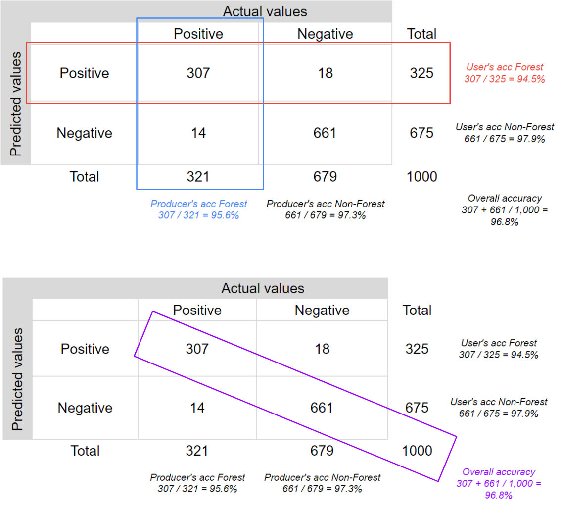
In this case, the classifier correctly identified 307 forest pixels, wrongly classified 18 non-forest pixels as forest, correctly identified 661 non-forest pixels, and wrongly classified 14 forest pixels as non-forest. Therefore, the classifier was correct 968 times and wrong 32 times. Let’s calculate the main accuracy metrics for this example.

The overall accuracy tells us what proportion of the reference data was classified correctly, and is calculated as the total number of correctly identified pixels divided by the total number of pixels in the sample.

In this case, the overall accuracy is 96.8%, calculated using (.

Two other important accuracy metrics are the producer’s accuracy and the user’s accuracy, also referred to as the “recall” and the “precision,” respectively. Importantly, these metrics quantify aspects of per-class accuracy.

The producer’s accuracy is the accuracy of the map from the point of view of the map maker (the “producer”), and is calculated as the number of correctly identified pixels of a given class divided by the total number of pixels actually in that class. The producer’s accuracy for a given class tells us the proportion of the pixels in that class that were classified correctly.

In this case, the producer’s accuracy for the forest class is 95.6%, calculated using ). The producer’s accuracy for the non-forest class is 97.3%, calculated from ).

The user’s accuracy (also called the “consumer’s accuracy”) is the accuracy of the map from the point of view of a map user, and is calculated as the number of correctly identified pixels of a given class divided by the total number of pixels claimed to be in that class. The user’s accuracy for a given class tells us the proportion of the pixels identified on the map as being in that class that are actually in that class on the ground.

In this case, the user’s accuracy for the forest class is 94.5%, calculated using ). The user’s accuracy for the non-forest class is 97.9%, calculated from ).

Fig. F2.2.1 helps visualize the rows and columns used to calculate each accuracy.

It is very common to talk about two types of error when addressing remote-sensing classification accuracy: omission errors and commission errors. Omission errors refer to the reference pixels that were left out of (omitted from) the correct class in the classified map. In a two-class system, an error of omission in one class will be counted as an error of commission in another class. Omission errors are complementary to the producer’s accuracy.

Commission errors refer to the class pixels that were erroneously classified in the map and are complementary to the user’s accuracy.

Finally, another commonly used accuracy metric is the kappa coefficient, which  evaluates how well the classification performed as compared to random. The value of the kappa coefficient can range from −1 to 1: a negative value indicates that the classification is worse than a random assignment of categories would have been; a value of 0 indicates that the classification is no better or worse than random; and a positive value indicates that the classification is better than random.

The chance agreement is calculated as the sum of the product of row and column totals for each class, and the observed accuracy is the overall accuracy. Therefore, for our example, the kappa coefficient is 0.927.

Now, let’s go back to the script. In Earth Engine, there are API calls for these operations. Note that our confusion matrix will be a 4 x 4 table, since we have four different classes.

Copy and paste the code below to classify the testingSet and get a confusion matrix using the method errorMatrix. Note that the classifier automatically adds a property called “classification,” which is compared to the “class” property of the reference dataset.

Copy and paste the code below to print the confusion matrix and accuracy metrics. Expand the confusion matrix object to inspect it. The entries represent the number of pixels. Items on the diagonal represent correct classification. Items off the diagonal are misclassifications, where the class in row i is classified as column j (values from 0 to 3 correspond to our class codes: forest, developed, water, and herbaceous, respectively). Also expand the producer’s accuracy, user’s accuracy (consumer’s accuracy), and kappa coefficient objects to inspect them.

How is the classification accuracy? Which classes have higher accuracy compared to the others? Can you think of any reasons why? (Hint: Check where the errors in these classes are in the confusion matrix—i.e., being committed and omitted.)

Code Checkpoint F22a. The book’s repository contains a script that shows what your code should look like at this point.

Section 2. Hyperparameter tuning

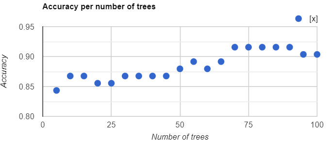
We can also assess how the number of trees in the Random Forest classifier affects the classification accuracy. Copy and paste the code below to create a function that charts the overall accuracy versus the number of trees used. The code tests from 5 to 100 trees at increments of 5, producing Fig. F2.2.2. (Do not worry too much about fully understanding each item at this stage of your learning. If you want to find out how these operations work, you can see more in Chaps. F4.0 and F4.1.)

Code Checkpoint F22b. The book’s repository contains a script that shows what your code should look like at this point.

Section 3. Spatial autocorrelation

We might also want to ensure that the samples from the training set are uncorrelated with the samples from the testing set. This might result from the spatial autocorrelation of the phenomenon being predicted. One way to exclude samples that might be correlated in this manner is to remove samples that are within some distance to any other sample. In Earth Engine, this can be accomplished with a spatial join. The following Code Checkpoint replicates Sect. 1 but with a spatial join that excludes training points that are less than 1000 meters distant from testing points.

Code Checkpoint F22c. The book’s repository contains a script that shows what your code should look like at this point.

Synthesis

Assignment 1. Based on Sect. 1, test other classifiers (e.g., a Classification and Regression Tree or Support Vector Machine classifier) and compare the accuracy results with the Random Forest results. Which model performs better?

Assignment 2. Try setting a different seed in the randomColumn method and see how that affects the accuracy results. You can also change the split between the training and testing sets (e.g., 70/30 or 60/40).

Conclusion

You should now understand how to calculate how well your classifier is performing on the data used to build the model. This is a useful way to understand how a classifier is performing, because it can help indicate which classes are performing better than others. A poorly modeled class can sometimes be improved by, for example, collecting more training points for that class.

Nevertheless, a model may work well on training data but work poorly in locations randomly chosen in the study area. To understand a model’s behavior on testing data, analysts employ protocols required to produce scientifically rigorous and transparent estimates of the accuracy and area of each class in the study region. We will not explore those practices in this chapter, but if you are interested, there are tutorials and papers available online that can guide you through the process. Links to some of those tutorials can be found in the “For Further Reading” section of this book.

Feedback

To review this chapter and make suggestions or note any problems, please go now to bit.ly/EEFA-review. You can find summary statistics from past reviews at bit.ly/EEFA-reviews-stats.

References

Congalton R (1994) Accuracy assessment of remotely sensed data: Future needs and directions. In: Proceedings of Pecora 12 land information from space-based systems. pp 385–388

Foody GM (2002) Status of land cover classification accuracy assessment. Remote Sens Environ 80:185–201. https://doi.org/10.1016/S0034-4257(01)00295-4

Olofsson P, Foody GM, Herold M, et al (2014) Good practices for estimating area and assessing accuracy of land change. Remote Sens Environ 148:42–57. https://doi.org/10.1016/j.rse.2014.02.015

Stehman SV (2013) Estimating area from an accuracy assessment error matrix. Remote Sens Environ 132:202–211. https://doi.org/10.1016/j.rse.2013.01.016

Stehman SV (1997) Selecting and interpreting measures of thematic classification accuracy. Remote Sens Environ 62:77–89. https://doi.org/10.1016/S0034-4257(97)00083-7

Stehman SV, Foody GM (2019) Key issues in rigorous accuracy assessment of land cover products. Remote Sens Environ 231:111199. https://doi.org/10.1016/j.rse.2019.05.018

Strahler AH, Boschetti L, Foody GM, et al (2006) Global land cover validation: Recommendations for evaluation and accuracy assessment of global land cover maps. Eur Communities, Luxemb 51:1–60

References

Cloud-Based Remote Sensing with Google Earth Engine. (n.d.). CLOUD-BASED REMOTE SENSING WITH GOOGLE EARTH ENGINE. https://www.eefabook.org/

Cloud-Based Remote Sensing with Google Earth Engine. (2024). In Springer eBooks. https://doi.org/10.1007/978-3-031-26588-4